CAPEX … IT’S PERSONAL

I built my first Telco Capex model back in 1999. I had just become responsible for what then was called Fixed Network Engineering with a portfolio of all technology engineering design & planning except for the radio access network but including all transport aspects from access up to Core and out to the external world. I got a bit frustrated that every time an assumption changed (e.g., business/marketing/sales), I needed to involve many people in my organization to revise their Capex demand. People that were supposed to get our greenfield network rolled out to our customers. Thus, I built a Capex model that would take the critical business assumptions, size my network (including the radio access network), and consistently assign the right Capex amounts to each category. The model allowed for rapid turnaround on revised business assumptions and a highly auditable track of changes, planning drivers, and unit prices. Since then, I have built best-practice Capex (and technology Opex) models for many Deutsche Telekom AGs and Ooredoo Group entities. Moreover, I have been creating numerous network and business assessment and valuation models (with an eye on M&A), focusing on technology drivers behind Capex and Opex for many different types of telco companies (30+) operating in an extensive range of market environments around the world (20+). Creating and auditing techno-economical models, making those operational and of high quality, it has (for me) been essential to be extensively involved operationally in the telecom sector.

PRELUDE TO CAPEX.

Capital investments, or Capital Expenditures, or just Capex for short, make Telcos go around. Capex is the monetary means used by your Telco to acquire, develop, upgrade, modernize, and maintain tangible, as well as, in some instances, intangible, assets and infrastructure. We can find Capex back under “Property, Plants, and Buildings” (or PPB) in a company’s balance sheet or directly in the profit & loss (or income) statement. Typically for an investment to be characterized as a capital expense, it needs to have a useful lifetime of at least 2 years and be a physical or tangible asset.

What about software? A software development asset is, by definition, intangible or non-physical. However, it can, and often is, assigned Capex status, although such an assignment requires a bit more judgment (and auditorial approvals) than for a real physical asset.

The “Modern History of Telecom” (in Europe) is well represented by Figure 1, showing the fixed-mobile total telecom Capex-to-Revenue ratio from 1996 to 2025.

From 1996 to 2012, most of the European Telco Capex-to-Revenue ratio was driven by investment into mobile technology introductions such as 2G (GSM) in 1996 and 3G (UMTS) in 2000 to 2002 as well as initial 4G (LTE) investments. It is clear that investments into fixed infrastructure, particularly modernizing and enhancing, have been down-prioritized only until recently (e.g., up to 2010+) when incumbents felt obliged to commence investing in fiber infrastructure and urgent modernization of incumbents’ fixed infrastructures in general. For a long time, the investment focus in the telecom industry was mobile networks and sweating the fixed infrastructure assets with attractive margins.

Figure 1 illustrates the “Modern History of Telecom” in Europe. It shows the historical development of Western Europe Telecom Capex to Revenue ratio trend from 1996 to 2025. The maximum was about 28% at the time 2G (GSM) was launched and at minimum after the cash crunch after ultra-expensive 3G licenses and the dot.com crash of 2020. In recent years, since 2008, Capex to Revenue has been steadily increasing as 4G was introduced and fiber deployment started picking up after 20210. It should be emphasized that the Capex to Revenue trend is for both Mobile and Fixed. It does not include frequency spectrum investments.

Across this short modern history of telecom, possibly one of the worst industry (and technology) investments have been the investments we did into 3G. In Europe alone, we invested 100+ billion Euro (i.e., not included in the Figure) into 2100 MHz spectrum licenses that were supposed to provide mobile customers “internet-in-their-pockets”. Something that was really only enabled with the introduction of 4G from 2010 onwards.

Also, from 2010 onwards, telecom companies (in Europe) started to invest increasingly in fiber deployment as well as upgrading their ailing fixed transport and switching networks focusing on enabling competitive fixed broadband services. But fiber investments have picked up in a significant way in the overall telecom Capex, and I suspect it will remain so for the foreseeable future.

Figure 2 When we take the European Telco revenue (mobile & fixed) over the period 1996 to 2025, it is clear that the mobile business model quantum leaped revenue from its inception to around 2008. After this, it has been in steady decline, even if improvement has been observed in the fixed part of the telco business due to the transition from voice-dominated to broadband. Source: https://stats.oecd.org/

As can be observed from Figure 1, since the telecom credit crunch between 2000 and 2003, the Capex share of revenue has steadily increased from just around 12% in 2004, right after the credit crunch, to almost 20% in 2021. Over the period from 2008 to 2021, the industry’s total revenue has steadily declined, as can be seen in Figure 2. Taking the last 10 years (2011-2021) of mobile and fixed revenue data has, on average, reduced by 4+ billion euros a year. The cumulative annual growth rate (CAGR) was at a great +6% from the inception of 2G services in 1996 to 2008, the year of the “great recession.” From 2008 until 2021, the CAGR has been almost -2% in annual revenue loss for Western Europe.

What does that mean for the absolute total Capex spend over the same period? Figure 3 provides the trend of mobile and fixed Capex spending over the period. Since the “happy days” of 2G and 3G Capex spending, Capex rapidly declined after the industry spent 100+ billion Euro on 3G spectrum alone (i.e., 800+ million euros per MHz or 4+ euros per MHz-pop) before the required multi-billion Euro in 3G infrastructure. Though, after 2009, which was the lowest Capex spend after the 3G licenses were acquired, the telecom industry has steadily grown its annual total Capex spend with ca. +1 billion Euro per year (up to 2021) financing new technology introductions (4G and 5G), substantial mobile radio and core modernizations (a big refresh ca. every 6 -7 years), increasing capacity to continuously cope with consumer demand for broadband, fixed transport, and core infrastructure modernization, and last but not least (since the last ~ 8 years) increasing focus on fiber deployment. Over the same period from 2009 to 2021, the total revenue has declined by ca. 5 billion euros per year in Western Europe.

Figure 3 Using the above “Total Capex to Revenue” (Figure 1) and “Total Revenue” (Figure 2) allows us to estimate the absolute “Total Capex” over the same period. Apart from the big Capex swing around the introduction of 2G and 3G and the sharp drop during the “credit crunch” (2000 – 2003), Capex has grown steadily whilst the industry revenue has declined.

It will be very interesting to see how the next 10 years will develop for the telecom industry and its capital investment. There is still a lot to be done on 5G deployment. In fact, many Telcos are just getting started with what they would characterize as “real 5G”, which is 5G standalone at mid-band frequencies (e.g., > 3 GHz for Europe, 2.5 GHz for the USA), modernizing antenna structures from standard passive (low-order) to active antenna systems with higher-order MiMo antennas, possible mmWave deployments, and of course, quantum leap fiber deployment in laggard countries in Europe (e.g., Germany, UK, Greece, Netherlands, … ). Around 2028 to 2030, it would be surprising if the telecoms industry would not commence aggressively selling the consumer the next G. That is 6G.

At this moment, the next 3 to 5 years of Capital spending are being planned out with the aim of having the 2024 budgets approved by November or December. In principle, the long-term plans, that is, until 2027/2028, have agreed on general principles. Though, with the current financial recession brewing. Such plans would likely be scrutinized as well.

I have, over the last year since I published this article, been asked whether I had any data on Ebitda over the period for Western Europe. I have spent considerable time researching this, and the below chart provides my best shot at such a view for the Telecom industry in Western Europe from the early days of mobile until today. This, however, should be taken with much more caution than the above Caex and Revenues, as individual Telco’ s have changed substantially over the period both in their organizational structure and how results have been represented in their annual reports.

Figure 4 illustrates the historical development of the EBITDA margin over the period from 1995 to 2022 and a projection of the possible trends from 2023 onwards.

IT’S THAT TIME OF THE YEAR … CAPEX IS IN THE AIR.

It is the time of the year when many telcos are busy updating their business and financial planning for the following years. It is not uncommon to plan for 3 to 5 years ahead. It involves scenario planning and stress tests of those scenarios. Scenarios would include expectations of how the relevant market will evolve as well as the impact of the political and economic environment (e.g., covid lockdowns, the war in Ukraine, inflationary pressures, supply-chain challenges, … ) and possible changes to their asset ownership (e.g., infrastructure spin-offs).

Typically, between the end of the third or beginning of the fourth quarter, telecommunications businesses would have converged upon a plan for the coming years, and work will focus on in-depth budget planning for the year to come, thus 2024. This is important for the operational part of the business, as work orders and purchase orders for the first quarter of the following year would need to be issued within the current year.

The planning process can be sophisticated, involving many parts of the organization considering many scenarios, and being almost mathematical in its planning nature. It can be relatively simple with the business’s top-down financial targets to adhere to. In most instances, it’s likely a combination of both. Of course, if you are a publicly-traded company or part of one, your past planning will generally limit how much your new planning can change from the old. That is unless you improve upon your old plans or have no choice but to disappoint investors and shareholders (typically, though, one can always work on a good story). In general, businesses tend to be cautiously optimistic about uncertain business drivers (e.g., customer growth, churn, revenue, EBITDA) and conservatively pessimistic on business drivers of a more certain character (e.g., Capex, fixed cost, G&A expenses, people cost, etc..). All that without substantially and negatively changing plans too much between one planning horizon to the next.

Capital expense, Capex, is one of the foundations, or enablers, of the telco business. It finances the building, expansion, operation, and maintenance of the telco network, allowing customers to enjoy mobile services, fixed broadband services, TV services, etc., of ever-increasing quality and diversity. I like to look at Capex as the investments I need to incur in order to sustain my existing revenues, grow my revenues (preferably beating inflationary pressures), and finance any efficiency activities that will reduce my operational expenses in the future.

If we want to make the value of Capex to the corporation a little firmer, we need a little bit of financial calculus. We can write a company’s value (CV) as

With g being the expected growth rate in free cash flow in perpetuity, WACC is the Weighted Average Cost of Capital, and FCFF is the Free Cash Flow to the Firm (i.e., company) that we can write as follows;

FCFF = NOPLAT + Depreciation & Amortization (DA) – ∆ Working Capital – Capex,

with NOPLAT being the Net Operating Profit Less Adjusted Taxes (i.e., EBIT – Cash Taxes). So if I have two different Capex budgets with everything else staying the same despite the difference in Capex (if true life would be so easy, right?);

assuming that everything except the proposed Capex remains the same. With a difference of, for example, 10 Million Euro, a future growth rate g = 0% (maybe conservative), and a WACC of 5% (note: you can find the latest average WACC data for the industry here, which is updated regularly by New York University Leonard N. Stern School of Business. The 5% chosen here serves as an illustration only. You should always choose the weighted average cost of capital that is applicable to your context). The above formula would tell us that the investment plan having 10 Million euros less would be 200 Million euros more valuable (20× the Capex not spent). Anyone with a bit of (hands-on!) experience in budget business planning would know that the above valuation logic should be taken with a mountain of salt. If you have two Capex plans with no positive difference in business or financial value, you should choose the plan with less Capex (and don’t count yourself rich on what you did not do). Of course, some topics may require Capex without obvious benefits to the top or bottom line. Such examples are easy to find, e.g., regulatory requirements or geo-political risks force investments that may appear valueless or even value destructive. Those require meticulous considerations, and timing may often play a role in optimizing your investment strategy around such topics. In some cases, management will create a narrative around a corporate investment decision that fits an optimized valuation, typically hedging on one-sided inflated risks to the business if not done. Whatever decision is made, it is good to remember that Capex, and resulting Opex, is in most cases a certainty. The business benefits in terms of more revenue or more customers are uncertain as is assuming your business will be worth more in a number of years if your antennas are yellow and not green. One may call this the “Faith-based case of more Capex.”

Figure 5 provides an overview of Western Europe of annual Fixed & Mobile Capex, Total and Service Revenues, and Capex to Revenue ratio (in %). Source: New Street Research Western Europe data.

Figure 5 provides an overview of Western European telcos’ revenue, Capex, and Capex to Revenue ratio. Over the last five years, Western European telcos have been spending increasingly higher Capex levels. In 2021 the telecom Capex was 6 billion euros higher than what was spent in 2017, about 13% higher. Fixed and mobile service revenue increased by 14 billion euros, yielding a Capex to Service revenue ratio of 23% in 2021 compared to 20.6% in 2017. In most cases, the total revenue would be reported, and if luck has its way (or you are a subscriber to New Street Research), the total Capex. Thus, capturing both the mobile and the fixed business, including any non-service-related revenues from the company. As defined in this article, non-service-related revenues would comprise revenues from wholesales, sales of equipment (e.g., mobile devices, STB, and CPEs), and other non-service-specific revenues. As a rule of thumb, the relative difference between total and service-related revenues is usually between 1.1 to 1.3 (e.g., the last 5-year average for WEU was 1.17). 

One of the main drivers for the Western European Capex has firstly been aggressive fiber-to-the-premise (FTTP) deployment, typically measured in homes passed across most of the European metropolitan footprint as well as urban areas in general. As fiber covers more and more residential households, increased subscription to fiber occurs as well. This also requires substantial additional Capex for a fixed broadband business. Figure 6 illustrates the annual FTTP (homes passed) deployment volume in Western Europe as well as the total household fiber coverage.

Figure 6 above shows the fiber to the premise (FTTP) home passed deployment per anno from 2017 to 2020 Actual (source: European Commission’s “Broadband Coverage in Europe 2020” authored by Omdia et al.) and 2021 to 2025 projected numbers (i.e., this author’s own assessment). During the period from 2017 to 2020, household fiber coverage grew from 24% to 37% and is expected to grow to at least 68% by 2025.

A large part of the initial deployment has been in relatively dense urban areas as well as relying on aerial fiber deployment outside bigger metropolitan centers. For example, in Portugal, with 82% of households covered with fiber as of 2020, the existing HFC infrastructure (duct, underground passageways, …) was a key enabler for the very fast, economical, and extensive household fiber coverage there. As the fiber rollout continues and even picks up pace towards 2025, I would expect to continue to see a substantial amount of Capex being attributed. In fact, what is often overlooked in the assessment of the Capex volume being committed to fiber deployment, is that the unit-Capex is likely to increase substantially as countries with no aerial deployment option pick up their fiber rollout pace (e.g., Germany, the UK, Netherlands) and countries with an already relatively high fiber coverage go increasingly suburban and rural.

The second main driver is in the domain of mobile network investment. The 5G radio access deployment has been a major driver in 2020 and 2021. It is expected to continue to contribute significantly to mobile operators Capex in the coming 5 years. For most Western European operators, the initial 5G deployment was at 700 MHz, which provides a very good 5G coverage. However, due to limited frequency spectral bandwidth, there are not very impressive speeds unless combined with a solid pre-existing 4G network. The deployment of 5G at 700 MHz has had a fairly modest effect on Mobile Capex (apart from what operators had to pay out in the 5G spectrum auctions to acquire the spectrum in the first place). Some mobile networks would have been prepared to accommodate the 700 MHz spectrum being supported by existing lower-order or classical antenna infrastructure. In 2021 and going forward, we will see an increasing part of the mobile Capex being allocated to 3.X GHz deployment. Far more sophisticated antenna systems, which co-incidentally also are far more costly in unit-Capex terms, will be taken into use, such as higher-order MiMo antennas from 8×8 passive MiMo to 32×32 and 64×64 active antennas systems. These advanced antenna systems will be deployed widely in metropolitan and urban areas. Some operators may even deploy these costly but very-high performing antenna systems in suburban and rural clutter with the intention to provide fixed-wireless access services to areas that today and for the next 5 – 7 years continue to be under-served with respect to fixed broadband fiber services.

Overall, I would also expect mobile Capex to continue to increase above and beyond the pre-2020 level.

As an external investor with little detailed insights into individual telco operations, it can be difficult to assess whether individual businesses or the industry are investing sufficiently into their technical landscape to allow for growth and increased demand for quality. Most publicly available financial reporting does not provide (if at all) sufficient insights into how capital expenses are deployed or prioritized across the many facets of a telco’s technical infrastructure, platforms, and services. As many telcos provide mobile and fixed services based on owned or wholesaled mobile and fixed networks (or combinations there off), it has become even more challenging to ascertain the quality of individual telecom operations capital investments.

Figure 7 illustrates why analysts like to plot Total Revenue against Total Capex (for fixed and mobile). It provides an excellent correlation. Though great care should be taken not to assume causation is at work here, i.e., “if I invest X Euro more, I will have Y Euro more in revenues.” It may tell you that you need to invest a certain level of Capex in sustaining a certain level of Revenue in your market context (i.e., country geo-socio-economic context). Source: New Street Research Western Europe data covering the following countries: AT, BE, DK, FI, FR, DE, GR, IT, NL, NO, PT, ES, SE, CH, and UK.

Why bother with revenues from the telco services? These would typically drive and dominate the capital investments and, as such, should relate strongly to the Capex plans of telcos. It is customary to benchmark capital spending by comparing the Capex to Revenue (see Figure 7), indicating how much a business needs to invest into infrastructure and services to obtain a certain income level. If nothing is stated, the revenue used for the Capex-to-Revenue ratio would be total revenue. For telcos with fixed and mobile businesses, it’s a very high-level KPI that does not allow for too many insights (in my opinion). It requires some de-averaging to become more meaningful.

THE TELCO TECHNOLOGY FACTORY

Figure 8 (below) illustrates the main capital investment areas and cost drivers for telecommunications operations with either a fixed broadband network, a mobile network, or both. Typically, around 90% of the capital expenditures will be invested into the technology factory comprising network infrastructure, products, services, and all associated with information technology. The remaining ca. 10% will be spent on non-technical infrastructures, such as shops, office space, and other non-tech tangible assets.

Figure 8 Telco Capex is spent across physical (or tangible) infrastructure assets, such as communications equipment, brick & mortar that hosts the equipment, and staff. Furthermore, a considerable amount of a telcos Capex will also go to human development work, e.g., for IT, products & services, either carried out directly by own staff or third parties (i.e., capitalized labor). The above illustrates the macro-levels that make out a mobile or fixed telecommunications network, and the most important areas Capex will be allocated to.

If we take the helicopter view on a telco’s network, we have the customer’s devices, either mobile devices (e.g., smartphone, Internet of Things, tablet, … ) or fixed devices, such as the customer premise equipment (CPE) and set-top box. Typically the broadband network connection to the customer’s premise would require a media converter or optical network terminator (ONT). For a mobile network, we have a wireless connection between the customer device and the radio access network (RAN), the cellular network’s most southern point (or edge). Radio access technology (e.g., 3G, 4G, or 5G) is very important determines for the customer experience. For a fixed network connection, we have fiber or coax (cable) or copper connecting the customer’s premise and the fixed network (e.g., street cabinet). Access (in general) follows the distribution of the customers’ locations and concentration, and their generated traffic is aggregated increasingly as we move north and up towards and into the core network. In today’s modern networks, big-fat-data broadband connections interconnect with the internet and big public data centers hosting both 3rd party and operator-provided content, services, and applications that the customer base demands. In many existing networks, data centers inside the operator’s own “walls” likewise will have service and application platforms that provide customers with more of the operator’s services. Such private data centers, including what is called micro data centers (μDCs) or edge DCs, may also host 3rd party content delivery networks that enable higher quality content services to a telco’s customer base due to a higher degree of proximity to where the customers are located compared to internet-based data centers (that could be located anywhere in the world).

Figure 9 illustrates break-out the details of a mobile as well as a fixed (fiber-based) network’s infrastructure elements, including the customers’ various types of devices.

Figure 9 illustrates that on a helicopter level, a fixed and a classical mobile network structure are reasonably similar, with the main difference of one network carrying the mobile traffic and the other the fixed traffic. The traffic in the fixed network tends to be at least ten larger than in the mobile network. They mainly differ in the access node and how it connects to the customer. For fixed broadband, the physical connection is established between, for example, the ONL (Optical Line Terminal) in the optical distribution network and ONT (Optical Line Terminal) at the customer’s home via a fiber line (i.e., wired). The wireless connection for mobile is between the Radio Node’s antenna and the end-user device. Note: AAS: Advanced Antenna System (e.g., MiMo, massive-MiMo), BBU: Base-band unit, CPE: Customer Premise Equipment, IOT: Internet of Things, IX: Internet Exchange, OLT: Optical Line Termination, and ONT: Optical Network Termination (same as ONU: Optical Network Unit).

From Figure 9 above, it should be clear that there are a lot of similarities between the mobile and fixed networks, with the biggest difference being that the mobile access network establishes a wireless connection to the customer’s devices versus the fixed access network physically wired connection to the device situated at the customer’s premises.

This is good news for fixed-mobile telecommunications operators as these will have considerable architectural and, thus, investment synergies due to those similarities. Although, the sad truth is that even today, many fixed-mobile telco companies, particularly incumbent, remain far away from having achieved fixed-mobile network harmonization and conversion.

Moreover, there are many questions to be asked as well as concerns when it comes to our industry’s Capex plans; what is the Capex required to accommodate data growth, are existing budgets allowing for sufficient network densification (to accommodate growth and quality), and what is the Capex trade-off between frequency spectrum acquisition, antenna technology, and site densification, how much Capex is justified to pursue the best network in a given market, what is the suitable trade-off between investing in fiber to the home and aggressive 5G deployment, should (incumbent) telco’s pursue fixed wireless access (FWA) and how would that impact their capital plans, what is the right antenna strategy, etc…

On a high level, I will provide guidance on many of the above questions, in this article and in forthcoming ones.

THE CAPEX STRUCTURE OF A TELECOM COMPANY.

When taking a macro look at Capex and not yet having a good idea about the breakdown between mobile and fixed investment levels, we are helped that on a macro level, the Capex categories are similar for a fixed and a mobile network. Apart from the last mile (access) in a fixed network is a fixed line (e.g., fiber, coax, or copper) and a wireless connection in a mobile network; the rest is comparable in nature and function. This is not surprising as a business with a fixed-mobile infrastructure would (should!) leverage the commonalities in transport and part of the access architecture.

In the fixed business, devices required to enable services on the fixed-line network at the fixed customers’ home (e.g., CPE, STB, …) are a capital expense driven by new customers and device replacement. This is not the case for mobile devices (i.e., an operational expense).

Figure 10 above illustrates the major Capex elements and their distribution defined by the median, lower and upper quantiles (the box), and lower and upper extremes (the whiskers) of what one should expect of various elements’ contribution to telco Capex. Note: CPE: Customer Premise Equipment, STB: Set-Top Box.

CUSTOMER PREMISE EQUIPMENT (CPE) & SET-TOP BOXES (STB) investments ARE between 10% to 20% of the TelEcoM Capex.

The capital investment level into Customer premise equipment (CPE) depends on the expected growth in the fixed customer base and the replacement of old or defective CPEs already in the fixed customer base. We would generally expect this to make out between 10% to 20% of the total Capex of a fixed-mobile telco (and 0% in a mobile-only business). When migrating from one access technology (e.g., copper/xDSL phase-out, coaxial cable) to another (e.g., fiber or hybrid coaxial cable), more Capex may be required. Similar considerations for set-top boxes (STB) replacement due to, for example, a new TV platform, non-compliance with new requirements, etc. Many Western European incumbents are phasing out their extensive and aging copper networks and replacing those with fiber-based networks. At the same time, incumbents may have substantial capital requirements phasing out their legacy copper-based access networks, the capital burden on other competitor telcos in markets where this is happening if such would have a significant copper-based wholesale relationship with the incumbent.

In summary, over the next five years, we should expect an increase in CPE-based Caped due to the legacy copper phase-out of incumbent fixed telcos. This will also increase the capital pressure in transport and access categories.

CPE & STB Capex KPIs: Capex share of Total and Capex per Gross Added Customer.

Capex modeling comment: Use your customer forecast model as the driver for new CPEs. Your research should give you an idea of the price range of CPEs used by your target fixed broadband business. Always include CPE replacement in the existing base and the gross adds for the new CPEs. Many fixed broadband retail businesses have been conservative in the capabilities of CPEs they have offered to their customer base (e.g., low-end cheaper CPEs, poor WiFi quality, ≤1Gbps), and it should be considered that these may not be sufficient for customer demand in the following years. An incumbent with a large install base of xDSL customers may also have a substantial migration (to fiber) cost as CPEs are required to be replaced with fiber cable CPEs. Due to the current supply chain and delivery issues, I would assume that operators would be willing to pay a premium for getting critical stock as well as having priority delivery as stock becomes available (e.g., by more expensive shipping means).

Core network & service platformS, including data centers, investments ARE between 8% to 12% of the telecom Capex.

Core network and service platforms should not take up more than 10% of the total Capex. We would regard anything less than 5% or more than 15% as an anomaly in Capital prioritization. This said, over the next couple of years, many telcos with mobile operations will launch 5G standalone core networks, which is a substantial change to the existing core network architecture. This also raises the opportunity for lifting and shifting from monolithic systems or older cloud frameworks to cloud-native and possibly migrating certain functions onto public cloud domains from one or more hyperscalers (e.g., AWS, Azure, Google). As workloads are moved from telco-owned data centers and own monolithic core systems, telco technology cost structure may change from what prior was a substantial capital expense to an operational expense. This is particularly true for software-related developments and licensing.

Another core network & service platform Capex pressure point may come from political or investor pressure to replace Chinese network elements, often far removed from obsolescence and performance issues, with non-Chinese alternatives. This may raise the Core network Capex level for the next 3 to 5 years, possibly beyond 12%. Alas, this would be temporary.

In summary, the following topics would likely be on the Capex priority list;

1. Life-cycle management investments (I like to call Business-as-Usual demand) into software and hardware maintenance, end-of-life replacements, growth (software licenses, HW expansions), and miscellaneous topics. This area tends to dominate the Capex demand unless larger transformational projects exist. It is also the first area to be de-prioritized if required. Working with Priority 1, 2, and 3 categorizations is a good Capital planning methodology. Where Priority 1 is required within the following budget year 1, Prio. 2 is important but can wait until year two without building up too much technical debt and Prio. 3 is nice to have and not expected to be required for the next two subsequent budget years.

2. 5G (Standalone, SA) Core Network deployment (timeline: 18 – 24 months).

3. Network cloudification, initially lift-and-shift with subsequent cloud-native transformation. The trigger point will be enabling the deployment of the 5G standalone (SA) core. Operators will also take the opportunity to clean up their data centers and network core location (timeline: 24 – 36 months).

4. Although edge computing data centers (DC) typically are supposed to support the radio access network (e.g., for Open-RAN), the capital assignment would be with the core network as the expertise for this resides here. The intensity of this Capex (if built by the operator, otherwise, it would be Opex) will depend on the country’s size and fronthaul/backhaul design. The investment trigger point would generally commence on Open-RAN deployment (e.g., 1&1 & Telefonica Germany). The edge DC (or μDC) would most like be standard container-sized (or half that size) and could easily be provided by independent towerco or specific edge-DC 3rd party providers lessening the Capex required for the telco. For smaller geographies (e.g., Netherlands, Denmark, Austria, …), I would not expect this item to be a substantial topic for the Capex plans. Mainly if Open-RAN is not being pursued over the next 5 – 10 years by mainstream incumbent telcos.

5. Chinese supplier replacement. The urgency would depend on regulatory pressure, whether compensation is provided (unlikely) or not, and the obsolescence timeline of the infrastructure in question. Given the high quality at very affordable economics, I expect this not to have the biggest priority and will be executed within timelines dictated more by economics and obsolescence timelines. In any case, I expect that before 2025 most European telcos will have phased out Chinese suppliers from their Core Networks, incl. any Service platforms in use today (timeline: max. 36 months).

6. Cybersecurity investments strengthen infrastructure, processes, and vital data residing in data centers, service platforms, and core network elements. I expect a substantial increase in Capex (and Opex) arising from the telco’s focus on increasing the cyber protection of their critical telecom infrastructure (timeline: max 18 months with urgency).

Core Capex KPIs: Capex share of Total (knowing the share, it is straightforward to get the Capex per Revenue related to the Core), Capex per Incremental demanded data traffic (in Gigabits and Gigabyte per second), Capex per Total traffic, Capex per customer.

Capex modeling comment: In case I have little specific information about an operator’s core network and service platforms, I would tend to model it as a Euro per Customer, Euro per-incremental customer, and Euro per incremental traffic. Checking that I am not violating my Capex range that this category would typically fall within (e.g., 8% to 12%). I would also have to consider obsolescence investments, taking, for example, a percentage of previous cumulated core investments. As mobile operators are in the process, or soon will be, of implementing a 5G standalone core, having an idea of the number of 5G customers and their traffic would be useful to factor that in separately in this Capex category.

Estimating the possible Capex spend on Edge-RAN locations, I would consider that I need ca. 1 μDC per 450 to 700 km2 of O-RAN coverage (i.e., corresponding to a fronthaul distance between the remote radio and the baseband unit of 12 to 15 km). There may be synergies between fixed broadband access locations and the need for μ-datacenters for an O-RAN deployment for an integrated fixed-mobile telco. I suspect that 3rd party towercos, or alike, may eventually also offer this kind of site solutions, possibly sharing the cost with other mobile O-RAN operators.

Transport – core, metro & aggregation investments are between 5% to 15% of Telecom Capex.

The transport network consists of an optical transport network (OTN) connecting all infrastructure nodes via optical fiber. The optical transport network extends down to the access layer from the Core through the Metro and Aggregation layers. On top, the IP network ensures logical connection and control flow of all data transported up and downstream between the infrastructure nodes. As data traffic is carried from the edge of the network upstream, it is aggregated at one or several places in the network (and, of course, disaggregated in the downstream direction). Thus, the higher the transport network, the more bandwidth is supported on the optical and the IP layers. Most of the Capex investment needs would ensure that sufficient optical and IP capacity is available, supporting the growth projections and new service requirements from the business and that no bottlenecks can occur that may have disastrous consequences on customer experience. This mainly comes down to adding cards and ports to the already installed equipment, upgrading & replacing equipment as it reaches capacity or quality limitations, or eventually becoming obsolete. There may be software license fees associated with growth or the introduction of new services that also need to be considered.

Figure 11 above illustrates (high-level) the transport network topology with the optical transport network and IP networking on top. Apart from optical and IP network equipment, this area often includes investments into IP application functions and related hardware (e.g., BNG, DHCP, DNS, AAA RADIUS Servers, …), which have not been shown in the above. In most cases, the underlying optical fiber network would be present and sufficiently scalable, not requiring substantial Capex apart from some repair and minor extensions. Note DWDM: Dense Wavelength-Division multiplexing is an optical fiber multiplexing technology that increases the bandwidth utilization of a FON, BNG: Border Network Gateway connecting subscribers to a network or an internet service providers (ISP) network, important in wholesale arrangements where a 3rd party provides aggregation and access. DHCP: Dynamic Host Configuration Protocol providing IP address allocation and client configurations. AAA: Authentication, Authorization, and Accounting of the subscriber/user, RADIUS: Remote Authentication Dial-In User Service (Server) providing the AAA functionalities.

Although many telcos operate fixed-mobile networks and might even offer fixed-mobile converged services, they may still operate largely separate fixed and mobile networks. It is not uncommon to find very different transport design principles as well as supplier landscapes between fixed and mobile. The maturity, when each was initially built, and technology roadmaps have historically been very different. The fixed traffic dynamics and data volumes are several times higher than mobile traffic. The geographical presence between fixed and mobile tends to be very different (unless the telco of interest is the incumbent with a considerable copper or HFC network). However, the biggest reason for this state of affairs has been people and technology organizations within the telcos resisting change and much more aggressive transport consolidation, which would have been possible.

The mobile traffic could (should!) be accommodated at least from the metro/aggregation layers and upstream through the core transport. There may even be some potential for consolidation on front and backhauls that are worth considering. This would lead to supplier consolidation and organizational synergies as the technology organizations converged into a fixed-mobile engineering organization rather than two separate ones.

I would expect the share of Capex to be on the higher end of the likely range and towards the 10+% at least for the next couple of years, mainly if fixed and mobile networks are being harmonized on the transport level, which may also create an opportunity reduce and harmonize the supplier landscape.

In summary, the following topics would likely be on the Capex priority list;

1. Life-cycle management (business-as-usual) investments, accommodating growth including new service and quality requirements (annual business-as-usual). There are no indications that the traffic or mobile traffic growth rate over the next five years will be very different from the past. If anything, the 5-year CAGR is slightly decreasing.
2. Consolidating fixed and mobile transport networks (timelines: 36 to 60 months, depending on network size and geography). Some companies are already in the process of getting this done.
3. Chinese supplier replacement. To my knowledge, there are fewer regulatory discussions and political pressure for telcos to phase out transport infrastructure. Nevertheless, with the current geopolitical climate (and the upcoming US election in 2024), telcos need to consider this topic very carefully; despite economic (less competition, higher cost), quality, and possible innovation, consequences may result in a departure from such suppliers. It would be a natural consideration in case of modernization needs. An accelerated phase-out may be justified to remove future risks arising from geopolitical pressures.

While I have chosen not to include the Access transport under this category, it is not uncommon to see its budget demand assigned to this category, as the transport side of access (fronthaul and backhaul transport) technically is very synergetic with the transport considerations in aggregation, metro, and core.

Transport Capex KPIs: Capex share of Total, the amount of Capex allocated to Mobile-only and Fixed-only (and, of course, to a harmonized/converged evolved transport network), The Utilization level (if data is available or modeled to this level). The amount of Capex-spend on fiber deployment, active and passive optical transport, and IP.

Capex modeling comment: I would see whether any information is available on a number of core data centers, aggregation, and metro locations. If this information is available, it is possible to get an impression of both core, aggregation, and metro transport networks. If this information is not available, I would assume a sensible transport topology given the particularities of the country where the operator resides, considering whether the operator is an incumbent fixed operator with mobile, a mobile-only operation, or a mobile operator that later has added fixed broadband to its product portfolio. If we are not talking about a greenfield operation, most, if not all, will already be in place, and mainly obsolescence, incremental traffic, and possible transport network extensions would incur Capex. It is important to understand whether fixed-mobile operations have harmonized and integrated their transport infrastructure or large-run those independently of each other. There is substantial Capex synergy in operating an integrated transport network, although it will take time and Capex to get to that integration point.

Access investments are typically between 35% to 50% of the Telecom Capex.

Figure 12 (above) is similar to Figure 8 (above), emphasizing the access part of Fixed and Mobile networks. I have extended the mobile access topology to capture newer development of Open-RAN and fronthaul requirements with pooling (“centralizing”) the baseband (BBU) resources in an edge cloud (e.g., container-sized computing center). Fronthaul & Open-RAN poses requirements to the access transport network. It can be relatively costly to transform a legacy RAN backhaul-only based topology to an Open-RAN fronthaul-based topology. Open-RAN and fronthaul topologies for Greenfield deployments are more flexible and at least require less Capex and Opex. 

Mobile Access Capex.

I will define mobile access (or radio access network, RAN) as everything from the antenna on the site location that supports the customers’ usage (or traffic demand) via the active radio equipment (on-site or residing in an edge-cloud datacenter), through the fronthaul and backhaul transport, up to the point before aggregation (i.e., pre-aggregation). It includes passive and active infrastructure on-site, steal & mortar or storage container, front- and backhaul transport, data center software & equipment (that may be required in an edge data center), and any other hardware or software required to have a functional mobile service on whatever G being sold by the mobile operator.

Figure 13 above illustrates a radio access network architecture that is typically deployed by an incumbent telco supporting up to 4G and 5G. A greenfield operation on 5G (and maybe 4G) could (maybe should?) choose to disaggregate the radio access node using an open interface, allowing for a supplier mix between the remote radio head (RRH and digital frontend) at the site location and the centralized (or distributed) baseband unit (BBU). Fronthaul connects the antenna and RRH with a remote BBU that is situated at an edge-cloud data center (e.g., storage container datacenter unit = micro-data center, μDC). Due to latency constraints, the distance between the remote site and the BBU should not be much more than 10 km. It is customary to name the 5G new radio node a gNB (g-Node-B) like the 4G radio node is named eNB (evolved-Node-B).

When considering the mobile access network, it is good to keep in mind that, at the moment, there are at least two main flavors (that can be mixed, of course) to consider. (1) A classical architecture with the site’s radio access hardware and software from a single supplier, with a remote radio head (RRH) as well as digital frontend processing at or near the antenna. The radio nodes do not allow for mixing suppliers between the remote RF and the baseband. Radio nodes are connected to backhaul transmission that may be enabled by fiber or microwave radios. This option is simple and very well-proven. However, it comes with supplier lock-in and possibly less efficient use of baseband resources as these are likewise fixed to the radio node that the baseband unit is installed. (2) A new Open- or disaggregated radio access network (O-RAN), with the Antenna and RHH at the site location, then connected via fronthaul (≤10 km distance) to a μDC that contains the baseband unit. The μDC would then be connected to the backhaul that connects northbound to aggregation and core. The open interface between the RRH (and digital frontend) and the BBU allows different suppliers and hosts the RAN-specific software on common off-the-shelf (COTS) computing equipment. It allows (in theory) for better scaling and efficiency with the baseband resources. However, the framework has not been standardized by the usual bodies of standardization (e.g., 3GPP) and is not universally accepted as a common standard that all telco suppliers would adhere to. It also has not reached maturity yet (sort of obvious) and is currently (as of July 2022) seen to be associated with substantial cyber-security risks (re: maturity). It may be an interesting deployment model for greenfield operations (e.g., Rakuten Mobile Japan, Jio India, 1&1 Germany, Dish Mobile USA).

For established incumbent mobile operators, I do not see Option (2) as very attractive, at least for the next 5 – 7 years when many legacy technologies (i.e., non-5G) remain to be supported. The main concern should be the maturity, lack of industry-wise standardization, as well as cost of transforming existing access transport networks into compliance with a fronthaul framework. Most likely, some incumbents, the “brave” ones, will deploy O-RAN for 1 or a few 5G bands and keep their legacy networks as is. Most incumbent mobile operators will choose (actually have chosen already) conventional suppliers and the classical topology option to provide their 5G radio access network as it has the highest synergy with the access infrastructure already deployed. Thus, if my assertion is correct, O-RAN will only start becoming mainstream in 5 to 7 years, when existing deployments become obsolete.

Planning the mobile-radio access networks Capex requirements is not (that) difficult. Most of it can be mathematically derived and be easily assessed against growth expectations, expected (or targeted) network utilization (or efficiency), and quality. The growth expectations (should) come from consumer and retail businesses’ forecast of mobile customers over the next 3 to 5 years, their expected usage (if they care, otherwise technology should), or data-plan distribution (maybe including technology distributions, if they care. Otherwise, technology should), as well as the desired level of quality (usually the best).

Figure 14 above illustrates a typical cellular planning structural hierarchy from the sector perspective. One site typically has 3 sectors. One sector can have multiple cells depending on the frequency bands installed in the (multi-band) antennas. Massive MiMo antenna systems provide target cellular beams toward the user’s device that extend the range of coverage (via the beam). Very fast scheduling will enable beams to be switched/cycled to other users in the covered sector (a bit oversimplified). Typically, the sector is planned according to the cell utilization, thus on a frequency-by-frequency basis.

Figure 15 illustrates that most investment drivers can be approached as statistical distributions. Those distributions will tell us how much investment is required to ensure that a critical parameter X remains below a pre-defined critical limit Xc within a given probability (i.e., the proportion of the distribution exceeding Xc). The planning approach will typically establish a reference distribution based on actual data. Then based on marketing forecasts, the planners will evolve the reference based on the expected future usage that drives the planning parameter. Example: Let X be the customer’s average speed in a radio cell (e.g., in a given sector of an antenna site) in the busy hour. The business (including technology) has decided it will target 98% of its cells and should provide better than 10 Mbps for more than 50% of the active time a customer uses a given cell. Typically, we will have several quality-based KPIs, and the more breached they are, the more likely it will be that a Capex action is initiated to improve the customer experience.

Network planners will have access to much information down to the cell level (i.e., the active frequency band in a given sector). This helps them develop solid planning and statistical models that provide confidence in the extrapolation of the critical planning parameters as demand changes (typically increases) that subsequently drive the need for expansions, parameter adjustments, and other optimization requirements. As shown in Figure 15 above, it is customary to allow for some cells to breach a defined critical limit Xc, usually though it is kept low to ensure a given customer experience level. Examples of planning parameters could be cell (and sector) utilization in the busy hour, active concurrent users in cell (or sector), duration users spend at a or lower deemed poor speed level in a given cell, physical resource block (the famous PRB, try to ask what it stands for & what it means😉) utilization, etc.

The following topics would likely be on the Capex priority list;

1. New radio access deployment Capex. This may be for building new sites for coverage, typically in newly built residential areas, and due to capacity requirements where existing sites can no longer support the demand in a given area. Furthermore, this Capex also covers a new technology deployment such as 5G or deploying a new frequency band requiring a new antenna solution like 3.X GHz would do. As independent tower infrastructure companies (towerco) increasingly are used to providing the required passive site infrastructure solution (e.g., location, concrete, or steel masts/towers/poles), this part will not be a Capex item but be charged as Opex back to the mobile operator. From a European mobile radio access network Capex perspective, the average cost of a total site solution, with active as well as passive infrastructure, should have been reduced by ca. 100 thousand plus Euro, which may translate into a monthly Opex charge of 800 to 1300 Euro per site solution. It should be noted that while many operators have spun off their passive site solutions to third parties and thus effectively reduced their site-related Capex, the cost of antennas has increased dramatically as operators have moved away from classical simple SiSo (Single-in Singe-out) passive antennas to much more advanced antenna systems supporting multiple frequency bands, higher-order antennas (e.g., MiMo) and recently also started deploying active antennas (i.e., integrated amplifiers). This is largely also driven by mobile operators commissioning more and more frequency bands on their radio-access sites. The planning horizon needs at least to be 2 years and preferably 3 to 5 years.
2. Capex investments that accommodate anticipated radio access growth and increased quality requirements. It is normal to be between 18 – 24 months ahead of the present capacity demand overall, accepting no more than 2% to 5% of cells (in BH) to breach a critical specification limit. Several such critical limits would be used for longer-term planning and operational day-to-day monitoring.
3. Life-cycle management (business-as-usual) investments such as software annual fees, including licenses that are typically structured around the technologies deployed (e.g., 2G, 3G, 4G, and 5G) and active infrastructure modernization replacing radio access equipment (e.g., baseband units, radio units, antennas, …) that have become obsolete. Site reworks or construction optimization would typically be executed (on request from the operator) by the Towerco entity, where the mobile operator leases the passive site infrastructure. Thus, in such instances may not be a Capex item but charged back as an Operational expense to the telco.
4. Even if there have been fewer regulatory discussions and political pressure for telcos to phase out radio access, Chinese supplier replacement should be considered. Nevertheless, with the current geopolitical climate (and the upcoming US election), telcos need to consider this topic very carefully; despite economic (less competition, higher cost), quality, and possible innovation, consequences may result in a departure from such suppliers. It would be a natural consideration in case of modernization needs. An accelerated phase-out may be justified to remove future risks arising from geopolitical pressures, although it would result in above-and-beyond capital commitment over a shorter period than otherwise would be the case. Telco valuation may suffer more in the short to medium term than otherwise would have been the case with a more natural phaseout due to obsolescence.

Mobile Access Capex KPIs: Capex share of Total, Access Utilization (reported/planned data traffic demand to the data traffic that could be supplied if all or part of the spectrum was activated), Capex per Site location, Capex per Incremental data traffic demand (in Gigabyte and Gigabit per second which is the real investment driver), Capex per Total Traffic (in Gigabyte and Gigabit per second), Capex per Mobile Customer and Capex to Mobile Revenue (preferably service revenue but the total is fine if the other is not available). As a rule of thumb, 50% of a mobile network typically covers rural areas, which also may carry less than 20% of the total data traffic.

Whether actual and planned Capex is available or an analyst is modeling it, the above KPIs should be followed over an extended period. A single year does not tell much of a story.

Capex modeling comment: When modeling the Capex required for the radio access network, you need to have an idea about how many sites your target telco has. There are many ways to get to that number. In most European countries, it is a matter of public record. Most telcos, nowadays, rarely build their own passive site infrastructure but get that from independent third-party tower companies (e.g., CellNex w. ca. 75k locations, Vantage Towers w. ca. 82k locations, … ) or site-share on another operators site locations if available. So, modeling the RAN Capex is a matter of having a benchmark of the active equipment, knowing what active equipment is most likely to be deployed and how much. I see this as being an iterative modeling process. Given the number of sites and historical Capex, it is possible to come to a reasonable estimate of both volumes of sites being changed and the range of unit-Capex (given good guestimates of active equipment pricing range). Of course, in case you are doing a Capex review, the data should be available to you, and the exercise is straightforward. The mobile Capex KPIs above will allow for consistency checks of a modeling exercise or guide a Capex review process.

I recommend using the classical topology described above when building a radio access model. That is unless you have information that the telco under analysis is transforming to a disaggregated topology with both fronthaul and backhaul. Remember you are not only required to capture the Capex for what is associated with the site location but also what is spent on the access transport. Otherwise, there is a chance that you over-estimate the unit-Capex for the site-related investments.

It is also worth keeping in mind that typically, the first place a telecom company would cut Capex (or down-prioritize) is pressured during the planning process would be in the radio access network category. The reason is that the site-related unitary capex tends to be incredibly well-defined. If you reduce your rollout to 100 site-related units, you should have a very well-defined quantum of Capex that can be allocated to another category. Also, the operational impact of cutting in this category tends to be very well-defined. Depending on how well planned the overall Capex has been done, there typically would be a slack of 5% to 10% overall that could be re-assigned or ultimately reduced if financial results warrant such a move.

Fixed Access Capex.

As mobile access, fixed access is about getting your service out to your customers. Or, if you are a wholesale provider, you can provide the means of your wholesale customer reaching their customer by providing your own fixed access transport infrastructure. Fixed access is about connecting the home, the office, the public institution (e.g., school), or whatever type of dwelling in general.

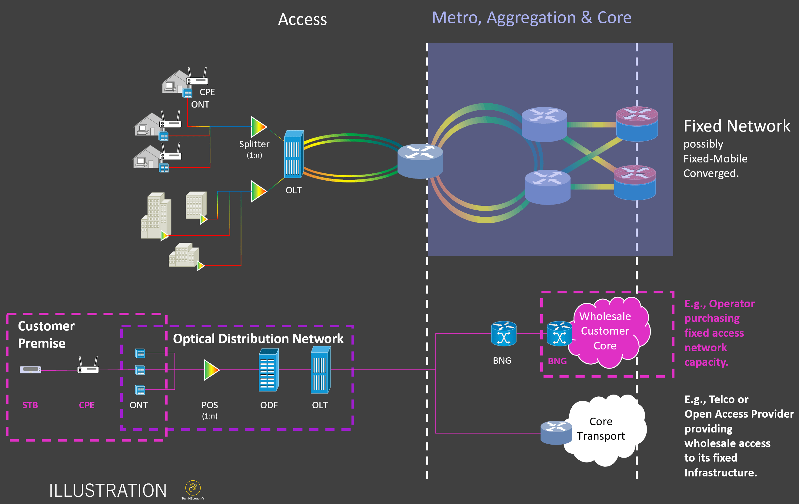
Figure 16 illustrates a fixed access network and its position in the overall telco architecture. The following make up the ODN (Optical Distribution Network); OLT: Optical Line Termination, ODF: Optical Distribution Frame, POS: Passive Optical Splitter, ONT: Optical Network Termination. At the customer premise, besides the ONT, we have the CPE: Customer Premise Equipment and the STB: Set-Top Box. Suppose you are an operator that bought wholesale fixed access from another telco’ (incl. Open Access Providers, OAPs). In that case, you may require a BNG to establish the connection with your customer’s CPE and STB through the wholesale access network.

As fiber optical access networks are being deployed across Europe, this tends to be a substantial Capex item on the budgets of telcos. Here we have two main Capex drivers. First is the Capex for deploying fibers across urban areas, which provides coverage for households (or dwellings) and is measured as Capex-per-homes passed. Second is the Capex required for establishing the connection to households (or dwellings). The method of fiber deployment is either buried, possibly using existing ducts or underground passageways, or via aerial deployment using established poles (e.g., power poles or street furniture poles) or new poles deployed with the fiber deployment. Aerial deployment tends to incur lower Capex than buried fiber solutions due to requiring less civil work. The OLT, ODF, POS, and optical fiber planning, design, and build to provide home coverage depends on the home-passed deployment ambition. The fiber to connect a home (i.e., civil work and materials), ONT, CPE, and STBs are driven by homes connected (or FTTH connected). Typically, CPE and STBs are not included in the Access Capex but should be accounted for as a separate business-driven Capex item.

The network solutions (BNG, OLT, Routers, Switches, …) outside the customer’s dwelling come in the form of a cabinet and appropriate cards to populate the cabinet. The cards provide the capacity and serviced speed (e.g., 100 Mbps, 300 Mbps, 1 Gbps, 10 Gbps, …) sold to the fixed broadband customer. Moreover, for some of the deployed solutions, there is likely a mandatory software (incl. features) fee and possibly both optional and custom-specific features (although rare to see that in mainstream deployments). It should be clear (but you would be surprised) that ONT and CPE should support the provisioned speed of the fixed access network. The customer cannot get more quality than the minimum level of either the ONT, CPE, or what the ODN has been built to deliver. In other words, if the networking cards have been deployed only to support up to 1 Gbps and your ONT, and CPE may support 3 Gbps or more, your customer will not be able to have a service beyond 1 Gbps. Of course, the other way around as well. I cannot stress enough the importance of longer-term planning in this respect. Your network should be as flexible as possible in providing customer services. It may seem that Capex savings can be made by only deploying capacity sold today or may be required by business over the next 12 months. While taking a 3 to 5-year view on the deployed network capacity and ONT/CPEs provided to customers avoids having to rip out relatively new equipment or finance the significant replacement of obsolete customer premise equipment that no longer can support the services required.

When we look at the economic drivers for fixed access, we can look at the capital cost of deploying a kilometer of fiber. This is particularly interesting if we are only interested in the fiber deployment itself and nothing else. Depending on the type of clutter, deployment, and labor cost occur. Maybe it is more interesting to bundle your investment into what is required to pass a household and what is required to connect a household (after it has been passed). Thus, we look at the Capex-per-home (or dwellings) passed and separate the Capex to connect an individual customer’s premise. It is important to realize that these Capex drivers are not just a single value but will depend on the household density depends on the type of area the deployment happens. We generally expect dense urban clutters to have a high dwelling density; thus, more households are covered (or passed) per km of fiber deployed. Dense-urban areas, however, may not necessarily hold the highest density of potential residential customers and hold less retail interest in the retail business. Generally, urban areas have higher household densities (including residential households) than sub-urban clutter. Rural areas are expected to have the lowest density and, thus, the most costly (on a household basis) to deploy.

Figure 17, just below, illustrates the basic economics of buried (as opposed to aerial) fiber for FTTH homes passed and FTTH homes connected. Apart from showing the intuitive economic logic, the cost per home passed or connected is driven by the household density (note: it’s one driver and fairly important but does not capture all the factors). This may serve as a base for rough assessments of the cost of fiber deployment in homes passed and homes connected as a function of household density. I have used data in the Fiber-to-the-Home Council Europe report of July 2012 (10 years old), “The Cost of Meeting Europe’s Network Needs” and have corrected for the European inflationary price increase since 2012 of ca. 14% and raised that to 20% to account for increased demand for FTTH related work by third parties. Then I checked this against some data points known to me (which do not coincide with the cities quoted in the chart). These data points relate to buried fiber, including the homes connected cost chart. Aerial fiber deployment (including home connected) would cost less than depicted here. Of course, some care should be taken in generalizing this to actual projects where proper knowledge of the local circumstances is preferred to the above.

Figure 17 The “chicken and egg” of connecting customers’ premises with fiber and providing them with 100s of Mbps up to Gbps broadband quality is that the fibers need to pass the home first, before the home can be connected. The cost of passing a premise (i.e., the home passed) and connecting a premise (home connected) should, for planning purposes, be split up. The cost of rolling out fiber to get homes-passed coverage is not surprisingly particularly sensitive to household density. We will have more households per unit area in urban areas compared to rural areas. Connecting a home is more sensitive to household density in deep rural areas where the distance from the main fiber line connection point to the household may be longer. The above cost curves are for buried fiber lines and are in 2021 prices.

Aerial fiber deployment would generally be less capital-intensive due to faster and easier deployment (less civil work, including permitting) using pre-existing (or newly built) poles. Not every country allows aerial deployment or even has the infrastructure (i.e., poles) available, which may be medium and low-voltage poles (e.g., for last-mile access). Some countries will have a policy allowing only buried fibers in the city or metropolitan areas and supporting pole infrastructure for aerial deployment in sub-urban and rural clutters. I have tried to illustrate this with Figure 18 below, where the pie charts show the aerial potential and share that may have to be assigned to buried fiber deployment.

Figure 18 above illustrates the amount of fiber coverage (i.e., in terms of homes passed) in Western European markets. The number for 2015 and 2020 is based on European Commission’s “Broadband Coverage in Europe 2020” (authored by Omdia et al.). The 2025 coverage number is my extrapolation of the 5-year trend leading up to 2020, considering the potential for aerial versus buried deployment. Aerial making accelerated deployment gains is more likely than in markets that only have buried fiber as a possibility, either because of regulation or lack of appropriate infrastructure for aerials. The only country that may be below 50% FTTH coverage in 2025 is Germany (i.e., DE), with a projected 39% of homes passed by 2025. Should Germany aim for 50% instead, they would have to do ca. 15 million households passed or, on average, 3 million a year from 2021 to 2025. Maximum Germany achieved in one year was in 2020, with ca. 1.4 million homes passed. The maximum any country in Europe has done in one year was France, with 2.9 million homes passed in 2018. However, France does allow for aerial fiber deployment outside major metropolitan areas.

Figure 19 above provides an overview across Western Europe for the last 5 years (2015 – 2020) of average annual household fiber deployment, the maximum done in one year in the previous 5 years, and the average required to achieve household coverage in 2025 shown above in Figure 13. For Germany (DE), the average deployment pace of 2.11 homes passed per year results in a coverage estimate of 39%. I don’t see any practical reasons for the UK, France, and Italy not to make the estimated household coverage by 2025, which may exceed my estimates.

From a deployment pace and Capex perspective, it is good to keep in mind that as time goes by, the deployment cost per household is likely to increase as household density reduces when the deployment moves from metropolitan areas toward suburban and rural. Thus, even if the deployment pace may reduce naturally for many countries in Figure 18 towards 2025, absolute Capex may not necessarily reduce accordingly.

In summary, the following topics would likely be on the Capex priority list;

1. Continued fiber deployment to achieve household coverage. Based on Figure 16, at household (HH) densities above 500 per km2, the unit Capex for buried fiber should be below 900 Euro per HH passed with an average of 600 Euro per HH passed. Below 500 HH per km2, the cost increases rapidly towards 3,000 Euro per HH passed. The aerial deployment will result in substantially lower Capex, maybe with as much as 50% lower unit Capex.
2. As customers subscribe, the fiber access cost associated with connecting homes (last-mile connectivity) will need to be considered. Figure 16 provides some guidance regarding the quantum-Euro range expected for buried fiber. Aerial-based connections may be somewhat cheaper.
3. Life-cycle management (business-as-usual) investments, modernization investments, accommodating growth including new service and quality requirements (annual business as usual). Typically it would be upgrading OLT, ONTs, routers, and switches to support higher bandwidth requirements upgrading line cards (or interface cards), and moving from ≤100 Mbps to 1 Gbps and 10 Gbps. Many telcos will be considering upgrading their GPON (Gigabit Passive Optical Networks, 2.5 Gbps↓ / 1.2 Gbps↑) to provide XGPON (10 Gbps↓ / 2.5 Gbps↑) or even XGSPON services (10 Gbps↓ / 10 Gbps↑).
4. Chinese supplier exposure and risks (i.e., political and regulatory enforcement) may be an issue in some Western European markets and require accelerated phase-out capital needs. In general, I don’t see fixed access infrastructure being a priority in this respect, given the strong focus on increasing household fiber coverage, which already takes up a lot of human and financial resources. However, this topic needs to be considered in case of obsolescence and thus would be a business case and performance-driven with a risk adjustment in dealing with Chinese suppliers at that point in time.

Fixed Access Capex KPIs: Capex share of Total, Capex per km, Number of HH passed and connected, Capex per HH passed, Capex per HH connected, Capex to Incremental Traffic, GPON, XGPON and XGSPON share of Capex and Households connected.

Whether actual and planned Capex is available or an analyst is modeling it, the above KPIs should be followed over an extended period. A single year does not tell much of a story.

Capex modeling comment: In a modeling exercise, I would use estimates for the telco’s household coverage plans as well as the expected household-connected sales projections. Hopefully, historical numbers would be available to the analyst that can be used to estimate the unit-Capex for a household passed and a household connected. You need to have an idea of where the telco is in terms of household density, and thus as time goes by, you may assume that the cost of deployment per household increases somewhat. For example, use Figure 17 to guide the scaling curve you need. The above-fixed access Capex KPIs should allow checking for inconsistencies in your model or, if you are reviewing a Capex plan, whether that Capex plan is self-consistent with the data provided.

If anyone would have doubted it, there is still much to do with fiber optical deployment in Western Europe. We still have around 100+ million homes to pass and a likely capital investment need of 100+ billion euros. Fiber deployment will remain a tremendously important investment area for the foreseeable future.

Figure 20 shows the remaining fiber coverage in homes passed based on 2020 actuals for urban and rural areas. In general, it is expected that once urban areas’ coverage has reached 80% to 90%, the further coverage-based rollout will reduce. Though, for attractive urban areas, overbuilt, that is, deploying fiber where there already are fibers deployed, is likely to continue.

Figure 21 illustrates the next 5 years’ weekly rollout to reach an 80% to 90% household coverage range by 2025. Further to the right, it shows an estimate of the remaining capital investment required to reach that 80% to 90% coverage range. This assessment is based on 2020 actuals from the European Commission’s “Broadband Coverage in Europe 2020” (authored by Omdia et al.); the weekly activity and Capex levels are thus from 2021 onwards.

In many Western European countries, the pace is expected to be increased considerably compared to the previous 5 years (i.e., 2015 – 2020). Even if the above figure may be over-optimistic, with respect to the goal of 2025, the European ambition for fiberizing European markets will impose a lot of pressure on speedy deployment.

IT investment levels are typically between 15% and 25% of Telecom Capex.

IT may be the most complex area to reach a consensus on concerning Capex. In my experience, it is also the area within a telco with the highest and most emotional discussion overhead within the operations and at a Board level. Just like everyone is far better at driving a car than the average driver, everyone is far better at IT than the IT experts and knows exactly what is wrong with IT and how to make IT much better and much faster, and much cheaper (if there ever was an area in telco-land where there are too many cooks).

Why is that the case? I tend to say that IT is much more “touchy-feely” than networks where most of the Capex can be estimated almost mathematically (and sufficiently complicated for non-technology folks to not bother with it too much … btw I tend to disagree with this from a system or architecture perspective). Of course, that is also not the whole truth.

IT designs, plans, develops (or builds), and operates all the business support systems that enable the business to sell to its customers, support its customers, and in general, keep the relationship with the customer throughout the customer life-cycle across all the products and services offered by the business irrespective of it being fixed or mobile or converged. IT has much more intense interactions with the business than any other technology department, whose purpose is to support the business in enabling its requirements.

Most of the IT Capex is related to people’s work, such as development, maintenance, and operations. Thus capitalized labor of external and internal labor is the main driver for IT Capex. The work relates to maintaining and improving existing services and products and developing new ones on the IT system landscape or IT stacks. In 2021, Western European telco Capex spending was about 20% of their total revenue. Out of that, 4±1 % or in the order of 10±3 billion Euro is spent on IT. With ca. 714 million fixed and mobile subscribers, this corresponds to an IT average spend of 14 Euros per telco customer in 2021. Best investment practices should aim at an IT Capex spend at or below 3% of revenue on average over 5 years (to avoid penalizing IT transformation programs). As a rule of thumb, if you do not have any details of internal cost structure (I bet you usually would not have that information), assume that the IT-related Opex has a similar quantum as Capex (you may compensate for GDP differences between markets). Thus, the total IT spend (Capex and Opex) would be in the order of 2×Capex, so the IT Spend to Revenue double the IT-related Capex to Revenue. While these considerations would give you an idea of the IT investment level and drill down a bit further into cost structure details, it is wise to keep in mind that it’s all a macro average, and the spread can be pretty significant. For example, two telcos with roughly the same number of customers, IT landscape, and complexity and have pretty different revenue levels (e.g., due to differences in ARPU that can be achieved in the particular market) may have comparable absolute IT spending levels but very different relative levels compared to the revenue. I also know of telcos with very low total IT spend to Revenue ITR (shareholder imposed), which had (and have) a horrid IT infrastructure performance with very extended outages (days) on billing and frequent instabilities all over its IT systems. Whatever might have been saved by imposing a dramatic reduction in the IT Capex (e.g., remember 10 million euros Capex reduction equivalent to 200 million euros value enhancement) was more than lost on inferior customer service and experience (including the inability to bill the customers).

You will find industry experts and pundits that expertly insist that your IT development spend is way too high or too low (although the latter is rare!). I recommend respectfully taking such banter seriously. Although try to understand what they are comparing with, what KPIs they are using, and whether it’s apples for apples and not with pineapples. In my experience, I would expect a mobile-only business to have a better IT spend level than a fixed-mobile telco, as a mobile IT landscape tends to be more modern and relatively simple compared to a fixed IT landscape. First, we often find more legacy (and I mean with a capital L) in the fixed IT landscape with much older services and products still being kept operational. The fixed IT landscape is highly customized, making transformation and modernization complex and costly. At least if old and older legacy products must remain operational. Another false friend in comparing one company IT spending with another’s is that the cost structure may be different. For example, it is worth understanding where OSS (Operational Support System) development is accounted for. Is it in the IT spend, or is it in the Network-side of things? Service platforms and Data Centers may be another difference where such spending may be with IT or Networks.

Figure 22 shows the helicopter view of a traditional telco IT architectural stack. Unless the telco is a true greenfield, it is a very normal state of affairs to have multiple co-existing stacks, which may have some degree of integration at various levels (sub-layers). Most fixed-mobile telcos remain with a high degree of IT architecture separation between their mobile and fixed business on a retail and B2B level. When approaching IT, investments never consider just one year. Understand their IT investment strategy in the immediate past (2-3 years prior) as well as how that fits with known and immediate future investments (2 – 3 years out).

Above, Figure 22 illustrates the typical layers and sub-layers in an IT stack. Every sub-layer may contain different applications, functionalities, and systems, all with an over-arching property of the sub-layer description. It is not uncommon for a telco to have multiple IT stacks serving different brands (e.g., value, premium, …) and products (e.g., mobile, fixed, converged) and business lines (e.g., consumer/retail, business-to-business, wholesale, …). Some layers may be consolidated across stacks, and others may be more fragmented. The most common division is between fixed and mobile product categories, as historically, the IT business support systems (BSS) as well as the operational support systems (OSS) were segregated and might even have been managed by two different IT departments (that kind of silliness is more historical albeit recent).

Figure 23 shows a typical fixed-mobile incumbent (i.e., anything not greenfield) multi-stack IT architecture and their most likely aspiration of aggressive integrated stack supporting a fixed-mobile conversion business. Out of experience, I am not a big fan of retail & B2B IT stack integration. It creates a lot of operational complexity and muddies the investment transparency and economics of particular B2B at the expense of the retail business

A typical IT landscape supporting fixed and mobile services may have quite a few IT stacks and a wide range of solutions for various products and services. It is not uncommon that a Fixed-Mobile telco would have several mobile brands (e.g., premium, value, …) and a separate (from an IT architecture perspective, at least) fixed brand. Then in addition, there may be differences between the retail (business-to-consumer, B2C) and the business-to-business (B2B) side of the telco, also being supported by separate stacks or different partitions of a stack. This is illustrated in Figure 20 above. In order for the telco business to become more efficient with respect to its IT landscape, including development, maintenance, and operational aspects of managing a complex IT infrastructure landscape, it should strive to consolidate stacks where it makes sense and not un-importantly along the business wish of convergence at least between fixed and mobile.

Figure 23 above illustrates an example of an IT stack harmonization activity long retail brands as well as Fixed and Mobile products as well as a separation of stacks into a retail and a business-to-business stack. It is, of course, possible to leverage some of the business logic and product synergies between B2C and B2B by harmonizing IT stacks across both business domains. However, in my experience, nothing great comes out of that, and more likely than not, you will penalize B2C by spending above and beyond value & investment attention on B2B. The B2B requirements tend to be significantly more complex to implement, their specifications change frequently (in line with their business customers’ demand), and the unit cost of development returns less unit revenue than the consumer part. Economically and from a value-consideration perspective, the telco needs to find an IT stack solution that is more in line with what B2B contributes to the valuation and fits its requirements. That may be a big challenge, particularly for minor players, as its business rarely justifies a standalone IT stack or developments. At least not a stack that is developed and maintained at the same high-quality level as a consumer stack. There is simply a mismatch in the B2B requirements, often having much higher quality and functionality requirements than the consumer part, and what it contributes to the business compared to, for example, B2C.

When I judge IT Capex, I care less about the absolute level of spend (within reason, of course) than what is practical to support within the given IT landscape the organization has been dealt with and, of course, the organization itself, including 3rd party support. Most systems will have development constraints and a natural order of how development can be executed. It will not matter how much money you are given or how many resources you throw at some problems; there will be an optimum amount of resources and time required to complete a task. This naturally leads to prioritization which may lead to disappointment of some stakeholders and projects that may not be prioritized to the degree they might feel entitled to.

When looking at IT capital spending and comparing one telco with another, it is worthwhile to take a 3- to 5-year time horizon, as telcos may be in different business and transformation cycles. A one-year comparison or benchmark may not be appropriate for understanding a given IT-spend journey and its operational and strategic rationale. Search for incidents (frequency and severity) that may indicate inappropriate spend prioritization or overall too little available IT budget.

The IT Capex budget would typically be split into (a) Consumer or retail part (i.e., B2C), (b) Business to Business and wholesale part, (c) IT technical part (optimization, modernization, cloudification, and transformations in general), and a (d) General and Administrative (G&A) part (e.g., Finance, HR, ..). Many IT-related projects, particularly of transformative nature, will run over multiple years (although if much more than 24 months, the risk of failure and monetary waste increases rapidly) and should be planned accordingly. For the business-driven demand (from the consumer, business, and wholesale), it makes sense to assign Capex proportional to the segment’s revenue and the customers those segments support and leverage any synergies in the development work required by the business units. For the IT part, capital spending should be assigned, ensuring that technical debt is manageable across the IT infrastructure and landscape and that efficiency gains arising from transformative projects (including landscape modernization) are delivered timely. In general, such IT projects promise efficiency in terms of more agile development possibilities (faster time to market), lower development and operational costs, and, last but not least, improved quality in terms of stability and reduced incidents. The G&A prioritizes finance projects and then HR and other corporate projects.

In summary, the following topics would likely be on the Capex priority list;

1. Provide IT development support for business demand in the next business plan cycle (3 – 5 years with a strong emphasis on the year ahead). The allocation key should be close to the Revenue (or Ebitda) and customer contribution expected within the budget planning period. The development focus is on maintenance, (incremental) improvements to existing products/services, and new products/services required to make the business plans. In my experience, the initial demand tends to be 2 to 3 times higher than what a reasonable financial envelope would dictate (i.e., even considering what is possible to do within the natural limitations of the given IT landscape and organization) and what is ultimately agreed upon.
2. Cloudification transformation journey moving away from the traditional monolithic IT platform and into a public, hybrid, or private cloud environment. The safest approach, in my opinion, is a “lift-and-shift” approach where existing functionality is developed in the cloud environment. After a successful migration from the traditional monolithic platform into the cloud environment, the next phase of the cloudification journey will be to move to a cloud-native framework should be embarked. This provides a very solid automation framework delivering additional efficiencies and improved stability and quality (e.g., reduction in incidents). Analysts should be aware that migrating to a (public) cloud environment may reduce the capitalization possibilities with the consequence that Capex may reduce in the forward budget planning, but this would be at the expense of increased Opex for the IT organization.
3. Stack consolidation. Reducing the number of IT stacks generally lowers the IT Capex demand and improves development efficiency, stability, and quality. The trend is to focus on the harmonization efforts on the frontend (Portals and Outlets layer in Figure 14), the CRM layer (retiring legacy or older CRM solutions), and moving down the layers of the IT stack (see Figure 14) often touching the complex backend systems when they become obsolete providing an opportunity to migrate to a modern cloud-based solution (e.g., cloud billing).
4. Modernization activities are not covered by cloudification investments or business requirements.
5. Development support for Finance (e.g., ERP/SAP requirements), HR requirements, and other miscellaneous activities not captured above.
6. Chinese suppliers are rarely an issue in Western European telecom’s IT landscape. However, if present in a telco’s IT environment, I would expect Capex has been allocated for phasing out that supplier urgently over the next 24 months (pending the complexity of such a transformation/migration program) due to strong political and regulatory pressures. Such an initiative may have a value-destructing impact as business-driven IT development (related to the specific system) might not be prioritized too highly during such a program and thus result in less ability to compete for the telco during a phase-out program.

IT Capex KPIs: IT share of Total Capex (if available, broken down into a Fixed and Mobile part), IT Capex to Revenue, ITR (IT total spend to Revenue), IT Capex per Customer, IT Capex per Employee, IT FTEs to Total FTEs.

Moreover, if available or being modeled, I would like to have an idea about how much of the IT Capex goes to investment categories such as (i) Maintain, (ii) Growth, and (iii) Transform. I will get worried if the majority of IT Capex over an extended period goes to the Growth category and little to Maintain and Transform. This indicates a telco that has deprioritized quality and ignores efficiency, resulting in the risk of value destruction over time (if such a trend were sustained). A telco with little Transform spend (again over an extended period) is a business that does not modernize (another word for sweating assets).

Capex modeling comment: when I am modeling IT and have little information available, I would first assume an IT Capex to Revenue ratio around 4% (mobile-only) to 6% (fixed-mobile operation) and check as I develop the other telco Capex components whether the IT Capex stays within 15% to 25%. Of course, keep an eye out for all the above IT Capex KPIs, as they provide a more holistic picture of how much confidence you can have in the Capex model.

Figure 24 Using New Street Research (total) Capex data for Western Europe and using the heuristics that IT spend typically would be 15% to 25% of the total Capex, we can estimate the most likely ranges of IT Capex to Revenue for the telecommunications business covered by NSR. For individual operations, we may also want to look at the time series of IT spending to revenue and compare that to any available intelligence (e.g., transformation intensive, M&A integration, business-as-usual, etc..)

Using the heuristic of the IT Capex being between 15% (1st quantile) and 25% (3rd quantile) of the total Capex, we can get an impression of how much individual Telcos invest in IT annually. The above chart shows such an estimate for 2021. I have the actual for several Western European Telcos, which agrees well with the above, typically a bit below the median.

Figure 25 having estimated the likely IT spend ranges for the various Western European telcos, allows us to estimate the IT spend per customer (using New Street Research data).

Similar to the IT Capex to Revenue, we can get an impression of what Telcos spend on IT Capex as it relates to their total mobile and fixed customer base. Again for Telcos in Western Europe (as well as outside), these ranges shown above do seem reasonable as the estimated range of where one would expect the IT spend.

Other, or miscellaneous, investments tend to be between 3% and 8% of the Telecom Capex.

When modeling a telco’s Capex, I find it very helpful to keep an “Other” or “Miscellaneous” Capex category for anything non-technology related. Modeling-wise, having a placeholder for items you don’t know about or may have forgotten is convenient. I typically start my models with 15% of all Capex. As my model matures, I should be able to reduce this to below 10% and preferably down to 5% (but I will accept 8% as a kind of good enough limit). I have had Capx review assignments where the Capex for future years had close to 20% in the “Miscellaneous.” If this “unspecified” Capex would not be included, the Capex to Revenue in the later years would drop substantially to a level that might not be deemed credible. In my experience, every planned Capex category will have a bit of “Other”-ness included as many smaller things require Capex but are difficult to mathematically derive a measure for. I tend to leave it if it is below 5% of a given Capex category. However, if it is substantial (>5%), it may reveal “sandbagging” or simply less maturity in the Capex planning and budget process.

Apart from a placeholder for stuff we don’t know, you will typically find Capex for shop refurbishment or modernization here, including office improvements and IT investments.

DE-AVERAGING THE TELECOM CAPEX TO FIXED AND MOBILE CONTRIBUTIONS.

There are similar heuristics to go deeper down into where the Capex should be spent, but that is a detail for another time.

Our first step is decomposing the total Capex into a fixed and a mobile component. We find that a multi-linear model including Total Capex, Mobile Customers, Mobile Service Revenue, Fixed Customers, and Fixed Service Revenues can account for 93% of the Capex trend. The multi-linear regression formula looks like the following;

with C = Capex, N = total customer count, R = service revenue, and α and β are the regression coefficient estimates from the multi-linear regression. The Capex model has been trained on 80% of the data (1,008 data points) chosen randomly and validated on the remainder (252 data points). All regression coefficients (4 in total) are statistically significant, with p-values well below a 95% confidence level.

Figure 26 above shows the Predicted Capex versus the Actual Capex. It illustrates that the predicted model agreed reasonably well with the actual Capex, which would also be expected based on the statistical KPIs resulting from the fit.

The Total is (obviously) available to us and therefore allows us to estimate both fixed and mobile Capex levels, by

The result of the fixed-mobile Capex decomposition is shown in Figure 26 below. Apart from being (reasonably) statistically sound, it is comforting that the trend in Capex for fixed and mobile seem to agree with what our intuition should be. The increase in mobile Capex (for Western Europe) over the last 5 years appears reasonable, given that 5G deployment commenced in early 2019. During the Covid lockdown from early 2020, fixed revenue was boosted by a massive shift in fixed broadband traffic (and voice) from the office to the individuals’ homes. Likewise, mobile service revenues have been in slow decline for years. Thus, the Capex increase due to 5G and reduced mobile service revenues ultimately leads to a relatively more significant increase in the mobile Capex to Revenue ratio.

Figure 27 illustrates the statistical modeling (by multi-linear regression), or decomposition, of the Total Capex as a function of Mobile Customers, Mobile Service Revenues, Fixed Customers, and Fixed Service Revenues, allowing to break up of the Capex into Fixed and Mobile components by decomposing the total Capex. The absolute Capex level is higher for fixed than what is found for mobile, with about a factor of 2 until 2021, when mobile Capex increases due to 5G investments in the mobile industry. It is found that the Mobile Capex has increased the most over the last 5 years (e.g., 5G deployment) while the service revenues have declined somewhat over the same period. This increased the Mobile Capex to Service Revenue ratio (note: based on Total Revenue, the ratio would be somewhat smaller, by ca. 17%). Source: Total Capex, Fixed, and Mobile Service revenues from New Street Research data for Western Europe. Note: The decomposition of the total Capex into Fixed and Mobile Capex is based on the author’s own statistical analysis and modeling. It is not a delivery of the New Street Research report.

CAN MOBILE-TRAFFIC GROWTH CONTINUE TO BE ACCOMMODATED CAPEX-WISE?

In my opinion, there has been much panic in our industry in the past about exhausting the cellular capacity of mobile networks and the imminent doom of our industry. A fear fueled by the exponential growth of user demand perceived inadequate spectrum amount and low spectral efficiency of the deployed cellular technologies, e.g., 3G-HSPA, classical passive single-in single-out antennas. Going back to the “hey-days” of 3G-HSPA, there was a fear that if cellular demand kept its growth rate, it would result in supply requirements going towards infinity and the required Capex likewise. So clearly an unsustainable business model for the mobile industry. Today, there is (in my opinion) no basis for such fears short or medium-term. With the increased fiberization of our society, where most homes will be connected to fiber within the next 5 – 10 years, cellular doomsday, in the sense of running out of capacity or needing infinite levels of Capex to sustain cellular demand, maybe a day never to come.

In Western Europe, the total mobile subscriber penetration was ca. 130% of the total population in 2021, with an excess of approximately 2.1+ mobile devices per subscriber. Mobile internet penetration was 76% of the total population in 2021 and is expected to reach 83% by 2025. In 2021, Europe’s average smartphone penetration rate was 77.6%, and it is projected to be around 84% by 2025. Also, by 2024±1, 50% of all connections in Western Europe are projected to be 5G connections. There are some expectations that around 2030, 6G might start being introduced in Western European markets. 2G and 3G will be increasingly phased out of the Western European mobile networks, and the spectrum will be repurposed for 4G and eventually 5G.

The above Figure 28 shows forecasted mobile users by their main mobile access technology. Source: based on the author’s forecast model relying on past technology diffusion trends for Western Europe and benchmarked against some WEU markets and other telco projections. See also 5G Standalone – European Demand & Expectations by Kim Larsen.

We may not see a complete phase-out of either older Gs, as observed in Figure 18. Due to a relatively large base of non-VOLTE (Voice-over-LTE) devices, mobile networks will have to support voice circuit-switched fallback to 2G or 3G. Furthermore, for the foreseeable future, it would be unlikely that all visiting roaming customers would have VOLTE-based devices. Furthermore, there might be legacy machine-2-machine businesses that would be prohibitively costly and complex to migrate from existing 2G or 3G networks to either LTE or 5G. All in all, ensure that 2G and 3G may remain with us for reasonably long.

Figure 29 above shows that mobile and fixed data traffic consumption is growing in totality and per-user level. On average mobile traffic grew faster than fixed from 2015 to 2021. A trend that is expected to continue with the introduction of 5G. Although the total traffic growth rate is slowing down somewhat over the period, on a per-user basis (mobile as well as fixed), the consumptive growth rate has remained stable.

Since the early days of 3G-HSPA (High-Speed Packet Access) radio access, investors and telco businesses have been worried that there would be an end to how much demand could be supported in our cellular networks. The “fear” is often triggered by seeing the exponential growth trend of total traffic or of the usage per customer (to be honest, that fear has not been made smaller by technology folks “panicking” as well).

Let us look at the numbers for 2021 as they are reported in the Cisco VNI report. The total mobile data traffic was in the order of 4 Exabytes (4 Billion gigabytes, GB), more than 5.5× the level of 2016. It is more than 600 million times the average mobile data consumption of 6.5 GB per month per customer (in 2021). Compare this with the Western European population of ca. 200 million. While big numbers, the 6.5 GB per month per customer is insignificant. Assuming that most of this volume comes from video streaming at an optimum speed of 3 – 5 Mbps (good enough for HD video stream), the 6.5 GB translates into approx. 3 – 5 hours of video streaming over a month.

The above Figure 30 Illustrates a 24-hour workday total data demand on the mobile network infrastructure. A weekend profile would be more flattish. We spend at least 12 hours in our home, ca. 7 hours at work (including school), and a maximum of 5 hours (~20%) commuting, shopping, and otherwise being away from our home or workplace. Previous studies of mobile traffic load have shown that 80% of a consumer’s mobile demand falls in 3 main radio node sites around the home and workplace. The remaining 20% tends to be much more mobile-like in the sense of being spread out over many different radio-node sites.

Daily we have an average of ca. 215 Megabytes per day (if spread equally over the month), corresponding to 6 – 10 minutes of video streaming. The average length of a YouTube was ca. 4.4 minutes. In Western Europe, consumers spend an average of 2.4 hours per day on the internet with their smartphones (having younger children, I am surprised it is not more than that). However, these 2.4 hours are not necessarily network-active in the sense of continuously demanding network resources. In fact, most consumers will be active somewhere between 8:00 to around 22:00, after which network demand reduces sharply. Thus, we have 14 hours of user busy time, and within this time, a Western European consumer would spend 2.4 hours cumulated over the day (or ca. 17% of the active time).

Figure 31 above illustrates (based on actual observed trends) how 5 million mobile users distribute across a mobile network of 5,000 sites (or radio nodes) and 15,000 sectors (typically 3 sectors = 1 site). Typically, user and traffic distributions tend to be log-norm-like with long tails. In the example above, we have in the busy hour a median value of ca. 80 users attached to a sector, with 15 being active (i.e., loading the network) in the busy hour, demanding a maximum of ca. 5 GB (per sector) or an average of ca. 330 MB per active user in the radio sector over that sector’s relevant busy hour.

Typically, 2 limits, with a high degree of inter-dependency, would allegedly hit the cellular businesses rendering profitable growth difficult at some point in the future. The first limit is a practical technology limit on how much capacity a radio access system can supply. As we will see a bit later, this will depend on the operator’s frequency spectrum position (deployed, not what might be on the shelf), the number of sites (site density), the installed antenna technology, and its effective spectral efficiency. The second (inter-dependent) limit is an economic limit. The incremental Capex that telcos would need to commit to sustaining the demand at a given quality level would become highly unprofitable, rendering further cellular business uneconomical.

From a Capex perspective, the cellular access part drives a considerable amount of the mobile investment demand. Together with the supporting transport, such as fronthaul, backhaul, aggregation, and core transport, the capital investment share is typically 50% or higher. This is without including the spectrum frequencies required to offer the cellular service. Such are usually acquired by local frequency spectrum auctions and amount to substantial investment levels.

In the following, the focus will be on cellular access.

Cellular Demand.

Before discussing the cellular supply side of things, let us first explore the demand side from the view of a helicopter. Demand is created by users (N) of the cellular services offered by telcos. Users can be human or non-human such as things in general or more specific machines. Each user has a particular demand that, in an aggregated way, can be represented by the average demand in Bytes per User (d). Thus, we can then identify two growth drivers. One from adding new users (ΔN) to our cellular network and another from the incremental change in demand per user (ΔN) as time goes by.

It should be noted that the incremental change in demand or users might not per se be a net increase. Still, it could also be a net decrease, either because the cellular networks have reached the maximum possible level of capacity (or quality) that results in users either reducing their demand or “ churning” from those networks or that an alternative to today’s commercial cellular network triggers abandonment as high-demand users migrate to that alternative — leading both to a reduction in cellular users and the average demand per user. For example, a near-100% Fiber-to-the-Home coverage with supporting WiFi could be a reason for users to abandon cellular networks, at least in an indoor environment, which would reduce between 60 to 80% of present-day cellular data demand. This last (hypothetical) is not an issue for today’s cellular networks and telco businesses.

Of course, this can easily be broken down into many more drivers and details, e.g., technology diffusion or adaptation, the rate of users moving from one access technology to another (e.g., 3G→4G, 4G→5G, 5G→FTTH+WiFi), improved network & user device capabilities (better coverage, higher speeds, lower latency, bigger display size, device chip generation), new cellular service adaptation (e.g., TV streaming, VR, AR, …), etc.…

However, what is often forgotten is that the data volume of consumptive demand (in Byte) is not the main direct driver for network demand and, thus, not for the required investment level. A gross volumetric demand can be caused by various gross throughput demands (bits per second). The throughput demanded in the busiest hour ( or ) is the direct driver of network load, and thus, network investments, the volumetric demand, is a manifestation of that throughput demand.

With being the number of active users in a given radio cell at the time-instant of unit t taken within a day.  is the Bytes consumed in a time instant (e.g., typically a second); thus, 8  gives us the bits per time unit (or bits/sec), which is throughput consumed. Sum over all the cells’ instant throughput ( bits/sec) in the same instant and take the maximum across. For example, a day provides the busiest hour throughput for the whole network. Each radio cell drives its capacity provision and supply (in bits/sec) and the investments required to provide that demanded capacity in the air interface and front- and back-haul.

For example, if n = 6 active (concurrent) users, each consuming on average  = 0.625 Mega Bytes per second (5 Megabits per second, Mbps), the typical requirement for a YouTube stream with an HD 1080p resolution, our radio access network in that cell would experience a demanded load of 30 Mbps (i.e., 6×5 Mbps). Of course, provided that the given cell has sufficient capacity to deliver what is demanded. A 4G cellular system, without any special antenna technology, e.g., Single-in-Single-out (SiSo) classical antenna and not the more modern Multiple-in-Multiple-out (MiMo) antenna, can be expected to deliver ca. 1.5 Mbps/MHz per cell. Thus, we would need at least 20 MHz spectrum to provide for 6 concurrent users, each demanding 5 Mbps. With a simple 2T2R MiMo antenna system, we could support about 8 simultaneous users under the same conditions. A 33% increase in what our system can handle without such an antenna. As mobile operators implement increasingly sophisticated antenna systems (i.e., higher-order MiMo systems) and move to 5G, a leapfrog in the handling capacity and quality will occur.

Figure 32 Is the sky the limit to demand? Ultimately, the limit will come from the practical and economic limits to how much can be supplied at the cellular level (e.g., spectral bandwidth, antenna technology, and software features …). Quality will reduce as the supply limit is reached, resulting in demand adaptation, hopefully settling at a demand-supply (metastable) equilibrium.

Cellular planners have many heuristics to work with that together trigger when a given radio cell would be required to be expanded to provide more capacity, which can be provided by software (licenses), hardware (expansion/replacement), civil works (sectorization/cell splits) and geographical (cell split) means. Going northbound, up from the edge of the radio network up through the transmission chain, such as fronthaul, back, aggregation, and core transport network, may require additional investments in expanding the supplied demand at a given load level.

As discussed, mobile access and transport together can easily make up more than half of a mobile capital budget’s planned and budgeted Capex.

So, to know whether the demand triggers new expansions and thus capital demand as well as the resulting operational expenses (Opex), we really need to look at the supply side. That is what our current mobile network can offer. When it cannot provide a targeted level of quality, how much capacity do we have to add to the network to be on a given level of service quality?

Cellular Supply.

Cellular capacity in units of throughput () given in bits per second, the basic building block of quality, is relatively easy to estimate. The cellular throughput (per unit cell) is provided by the amount of committed frequency spectrum to the air interface, what your radio access network and antenna support are, multiplied by the so-called spectral efficiency in bits per Hz per cell. The spectral efficiency depends on the antenna technology and the underlying software implementation of signal processing schemes enabling the details of receiving and sending signals over the air interface.

$T_{supply}$ can be written as follows;

With Mbps being megabits (a million bits) per second and MHz being Mega Herz.

For example, if we have a site that covers 3 cells (or sectors) with a deployed 100 MHz @ 3.6GHz (B) on a 32T32R advanced antenna system (AAS) with an effective downlink (i.e., from the antenna to user), spectral efficiency of ca. 20 Mbps/MHz/cell (i.e., ), we should expect to have a cell throughput on average at 1,000 Mbps (1 Gbps).

The capacity supply formula can be applied to the cell-level consideration providing sizing and thus investment guidance as we move northbound up the mobile network and traffic aggregates and concentrates towards the core and connections points to the external internet.

From the demand planning (e.g., number of customers, types of services sold, etc..), that would typically come from the Marketing and Sales department within the telco company, the technical team can translate those plans into a network demand and then calculate what they would need to do to cope with the customer demand within an agreed level of quality.

In Figure 33 above, operators provide cellular capacity by deploying their spectral assets on an appropriate antenna type and system-level radio access network hardware and software. Competition can arise from a superior spectrum position (balanced across low, medium, and high-frequency bands), better or more aggressive antenna technology, and utilizing their radio access supplier(s)’ features (e.g., signal processing schemes). Usually, the least economical option will be densifying the operator’s site grid where needed (on a macro or micro level).

Figure 34 above shows the various options available to the operator to create more capacity and quality. In terms of competitive edge, more spectrum than competitors provided it is being used and is balanced across low, medium, and high bands, provides the surest path to becoming the best network in a given market, and be difficult to economically copy by operators with substantially less spectrum. Their options would be compensating for the spectrum deficit by building more sites and deploying more aggressive antenna technologies. The last one is relatively easy to follow by anyone and may only provide some respite temporarily.  

An average mobile network in Western Europe has ca. 270 MHz spectrum (60 MHz low-band below 1800 and 210 MHz medium-band below 5 GHz) distributed over an average of 7 cellular frequency bands. It is rare to see all bands deployed in actual deployments and not uniformly across a complete network. The amount of spectrum deployed should match demand density; thus, more spectrum is typically deployed in urban areas than in rural ones. In demand-first-driven strategies, the frequency bands will be deployed based on actual demand that would typically not require all bands to be deployed. This is opposed to MNOs that focus on high quality, where demand is less important and where typically, most bands would be deployed extensively across their networks. The demand-first-driven strategy tends to be the most economically efficient strategy as long as the resulting cellular quality is market-competitive and customers are sufficiently satisfied.

In terms of downlink spectral capacity, we have an average of 155 MHz or 63 MHz, excluding the C-band contribution. Overall, this allows for a downlink supply of a minimum of 40 GB per hour (assuming low effective spectral efficiency, little advanced antenna technology deployed, and not all medium-band being utilized, e.g., C-Band and 2.5 GHz). Out of the 210 MHz mid-band spectrum, 92 MHz falls in the 3.X GHz (C-band) range and is thus still very much in the process of being deployed for 5G (as of June 2022). The C-band has, on average, increased the spectral capacity of Western European telcos by 50+% and, with its very high suitability for deployment together with massive MiMo and advanced antenna systems, effectively more than doubled the total cellular capacity and quality compared to pre-C-band deployment (using a 64T64R massive MiMo as a reference with today’s effective spectral efficiency … it will be even better as time goes by).

Figure 35 (above) shows the latest Ookla and OpenSignal DL speed benchmarks for Western Europe MNOs (light blue circles), and comparing this with their spectrum holdings below 3.x GHz indicates that there may be a lot of unexploited cellular capacity and quality to be unleashed in the future. Although, it would not be for free and likely require substantial additional Capex if deemed necessary. The ‘Expected DL Mbps’ (orange solid line, *) assumes the simplest antenna setup (e.g., classical SiSo antennas) and that all bands are fully used. On average, MNOs above the benchmark line have more advanced antenna setups (higher-order antennas) and fully (or close to) spectrum deployment. MNOs below the benchmark line likely have spectrum assets that have not been fully deployed yet and (or) “under-prioritized” their antenna technology infrastructure. The DL spectrum holding excludes C- and mmWave spectrum. Note:  There was a mistake in the original chart published on LinkedIn as the data was depicted against the total spectrum holding (DL+UL) and not only DL. Data: 54 Western European telcos.

Figure 35 illustrates the Western European cellular performance across MNOs, as measured by DL speed in Mbps, and compares this with the theoretical estimate of the performance they could have if all DL spectrum (not considering C-band, 3.x GHz) in their portfolio had been deployed at a fairly simple antenna setup (mainly SiSo and some 2T2R MiMo) with an effective spectral efficiency of 0.85 Mbps per MHz. It is good to point out that this is expected of 3G HSPA without MiMo. We observe that 21 telcos are above the solid (orange) line, and 33 have an actual average measured performance that is substantially below the line in many cases. Being above the line indicates that most spectrum has been deployed consistently across the network, and more advanced antennas, e.g., higher-order MiMo, are in use. Being below the line does (of course) not mean that networks are badly planned or not appropriately optimized. Not at all. Choices are always made in designing a cellular network. Often dictated by the economic reality of a given operator, geographical demand distribution, clutter particularities, or the modernization cycle an operator may be in. The most obvious reasons for why some networks are operating well under the solid line are; (1) Not all spectrum is being used everywhere (less in rural and more in urban clutter), (2) Rural configurations are simpler and thus provide less performance than urban sites. We have (in general) more traffic demand in urban areas than in rural. Unless a rural area turns seasonally touristic, e.g., lake Balaton in Hungary in the summer … It is simply a good technology planning methodology to prioritize demand in Capex planning, and it makes very good economic sense (3) Many incumbent mobile networks have a fundamental grid based on (GSM) 900MHz and later in-filled for (UMTS) 2100MHz…which typically would have less site density than networks based on (DCS) 1800MHz. However, site density differences between competing networks have been increasingly leveled out and are no longer a big issue in Western Europe (at least).

Overall, I see this as excellent news. For most mobile operators, the spectrum portfolio and the available spectrum bandwidth are not limiting factors in coping with demanded capacity and quality. Operators have many network & technology levers to work with to increase both quality and capacity for their customers. Of course, subject to a willingness to prioritize their Capex accordingly.

A mobile operator has few options to supply cellular capacity and quality demanded by its customer base.

• Acquire more spectrum bandwidth by buying in an auction, buying from 3rd party (including M&A), asymmetric sharing, leasing, or trading (if regulatory permissible).
• Deploy a better (spectral efficient) radio access technology, e.g., (2G, 3G) → (4G, 5G) or/and 4G → 5G, etc. Benefits will only be seen once a critical mass of customer terminal equipment supporting that new technology has been reached on the network (e.g., ≥20%).
• Upgrade antenna technology infrastructure from lower-order passive antennas to higher-order active antenna systems. In the same category would be to ensure that smart, efficient signal processing schemes are being used on the air interface.
• Building a denser cellular network where capacity demand dictates or coverage does not support the optimum use of higher frequency bands (e.g., 3.x GHz or higher).
• Small cell deployment in areas where macro-cellular built-out is no longer possible or prohibitively costly. Though small cells scale poorly with respect to economics and maybe really the last resort.

Sectorization with higher-frequency massive-MiMo may be an alternative to small-cell and macro-cellular additions. However, sectorization requires that it is possible civil-engineering wise (e.g., construction) re: structural stability, permissible by the landlord/towerco and finally economic compared to a new site built. Adding more than the usual 3-sectors to a site would further boost site spectral efficiency as more antennas are added.

Acquiring more spectrum requires that such spectrum is available either by a regulatory offering (public auction, public beauty contest) or via alternative means such as 3rd party trading, leasing, asymmetric sharing, or by acquiring an MNO (in the market) with spectrum. In Western Europe, the average cost of spectrum is in the ballpark of 100 million Euro per 10 million population per 20 MHz low-band or 100 MHz medium bands. Within the European Union, recent auctions provide a 20-year usage-rights period before the spectrum would have to be re-auctioned. This policy is very different from, for example, in the USA, where spectrum rights are bought and ownership secured in perpetuity (sometimes conditioned on certain conditions being met). For Western Europe, apart from the mmWave spectrum, in the foreseeable future, there will not be many new spectrum acquisition opportunities in the public domain.

This leaves mobile operators with other options listed above. Re-farming spectrum away from legacy technology (e.g., 2G or 3G) in support of another more spectral efficient access technology (e.g., 4G and 5G) is possibly the most straightforward choice. In general, it is the least costly choice provided that more modern options can support the very few customers left. For either retiring 2G or 3G, operators need to be aware that as long as not all terminal equipment support Voice-over-LTE (VoLTE), they need to keep either 2G or 3G (but not both) for 4G circuit-switched fallback (to 2G or 3G) for legacy voice services. The technologist should be prepared for substantial pushback from the retail and wholesale business, as closing down a legacy technology may lead to significant churn in that legacy customer base. Although, in absolute terms, the churn exposure should be much smaller than the overall customer base. Otherwise, it will not make sense to retire the legacy technology in the first place. Suppose the spectral re-farming is towards a new technology (e.g., 5G). In that case, immediate benefits may not occur before a critical mass of capable devices is making use of the re-farmed spectrum. The Capex impact of spectral re-farming tends to be minor, with possibly some licensing costs associated with net savings from retiring the legacy. Most radio departments within mobile operators, supplier experts, and managed service providers have gained much experience in this area over the last 5 – 7 years.

Another venue that should be taken is upgrading or modernizing the radio access network with more capable antenna infrastructure, such as higher-order massive MiMo antenna systems. As has been pointed out by Prof. Emil Björnson also, the available signal processing schemes (e.g., for channel estimation, pre-coding, and combining) will be essential for the ultimate gain that can be achieved. This will result in a leapfrog increase in spectral efficiency. Thus, directly boosting air-interface capacity and the quality that the mobile customer can enjoy. If we take a 20-year period, this activity is likely to result in a capital demand in the order of 100 million euros for every 1,000 sites being modernized and assumes a modernization (or obsolescence) cycle of 7 years. In other words, within the next 20 years, a mobile operator will have undergone at least 3 antenna-system modernization cycles. It is important to emphasize that this does not (entirely) cover the likely introduction of 6G during the 20 years. Operators face two main risks in their investment strategy. One risk is that they take a short-term look at their capital investments and customer demand projections. As a result, they may invest in insufficient infrastructure solutions to meet future demands, forcing accelerated write-offs and re-investments. The second significant risk is that the operator invests too aggressively upfront in what appears to be the best solution today to find substantially better and more efficient solutions in the near future that more cautious competitive operators could deploy and achieve a substantially higher quality and investment efficiency. Given the lack of technology maturity and the very high pace of innovation in advanced antenna systems, the right timing is crucial but not straightforward.

Last and maybe least, the operator can choose to densify its cellular grid by adding one or more macro-cellular sites or adding small cells across existing macro-cellular coverage. Before it is possible to build a new site or site, the operator or the serving towerco would need to identify suitable locations and subsequently obtain a permit to establish the new site or site. In urban areas, which typically have the highest macro-site densities, getting a new permit may be very time-consuming and with a relatively high likelihood of not being granted by the municipality. Small cells may be easier to deploy in urban environments than in macro sites. For operators making use of towerco to provide the passive site infrastructure, the cost of permitting and building the site and materials (e.g., steel and concrete) is a recurring operational expense rather than a Capex charge. Of course, active equipment remains a Capex item for the relevant mobile operator.

The conclusion I make above is largely consistent with the conclusions made by New Street Research in their piece “European 5G deep-dive” (July 2021). There is plenty of unexploited spectrum with the European operators and even more opportunity to migrate to more capable antenna systems, such as massive-MiMo and active advanced antenna systems. There are also above 3GHz, other spectrum opportunities without having to think about millimeter Wave spectrum and 5G deployment in the high-frequency spectrum range.

ACKNOWLEDGEMENT.

I greatly acknowledge my wife Eva Varadi, for her support, patience, and understanding during the creative process of writing this Blog. There should be no doubt that without the support of Russell Waller (New Street Research), this blog would not have been possible. Thank you so much for providing much of the data that lays the ground for much of the Capex analysis in this article. Of course, a lot of thanks go out to my former Technology and Network Economics colleagues, who have been a source of inspiration and knowledge. I cannot get away with acknowledging Maurice Ketel (who for many years let my Technology Economics Unit in Deutsche Telekom, I respect him above and beyond), Paul Borker, David Haszeldine, Remek Prokopik, Michael Dueser, Gudrun Bobzin, as well as many, many other industry colleagues who have contributed with valuable insights, discussions & comments throughout the years. Many thanks to Paul Zwaan for a lot of inspiration, insights, and discussions around IT Architecture.

Without executive leadership’s belief in the importance of high-quality techno-financial models, I have no doubt that I would not have been able to build up the experience I have in this field. I am forever thankful, for the trust and for making my professional life super interesting and not just a little fun, to Mads Rasmussen, Bruno Jacobfeuerborn, Hamid Akhavan, Jim Burke, Joachim Horn, and last but certainly not least, Thorsten Langheim.

FURTHER READING.

1. Kim Kyllesbech Larsen, “5G Standalone European Demand Expectations (Part I).”, (January, 2022).
2. Kim Kyllesbech Larsen, “RAN Unleashed … Strategies for being the best (or the worst) cellular network (Part III).”, (January, 2022).
3. Tom Copeland, Tim Koller, and Jack Murrin, “Valuation”, John Wiley & Sons, (2000). I regard this as my “bible” when it comes to understanding enterprise valuation. There are obviously many finance books on valuation (I have 10 on my bookshelf). Copeland’s book is the best imo.
4. Stefan Rommer, Peter Hedman, Magnus Olsson, Lars Frid, Shabnam Sultana, and Catherine Mulligan, “5G Core Networks”, Academic Press, (2020, 1st edition). Good account for what a 5G Core Network entails.
5. Jia Shen, Zhongda Du, Zhi Zhang, Ning Yang and Hai Tang, “5G NR and enhancements”, Elsevier (2022, 1st edition). Very good and solid account of what 5G New Radio (NR) is about and the considerations around it.
6. Wim Rouwet, “Open Radio Access Network (O-RAN) Systems Architecture and Design”, Academic Press, (2022). One of the best books on Open Radio Access Network architecture and design (honestly, there are not that many books on this topic yet). I like that the author, at least as an introduction makes the material reasonably accessible to even non-experts (which tbh is also badly needed).
7. Strand Consult, “OpenRAN and Security: A Literature Review”, (June, 2022). Excellent insights into the O-RAN maturity challenges. This report focuses on the many issues around open source software-based development that is a major part of O-RAN and some deep concerns around what that may mean for security if what should be regarded as critical infrastructure. I warmly recommend their “Debunking 25 Myths of OpenRAN”.
8. Hwaiyu Geng P.E., “Data Center Handbook”, Wiley (2021, 2nd edition). I have several older books on the topic that I have used for my models. This one brings the topic of data center design up to date. Also includes the topic of Cloud and Edge computing. Good part on Data Center financial analysis. 
9. James Farmer, Brian Lane, Kevin Bourgm Weyl Wang, “FTTx Networks, Technology Implementation, and Operations”, Elsevier, (2017, 1st edition). It has some books covering FTTx deployment, GPON, and other alternative fiber technologies. I like this one in particular as it covers hands-on topics as well as basic technology foundations.
10. Tower companies overview, “Top-12 Global 5G Cell Tower Companies 2021”, (Nov. 2021). A good overview of international tower companies with a meaningful footprint in Europe.
11. New Street Research, “European 5G deep-dive”, (July, 2021).
12. Prof. Emil Björnson, https://ebjornson.com/research/ and references therein. Please take a look at many of Prof. Björnson video presentations (e.g., many brilliant YouTube presentations that are fairly assessable).