5G Economics – An Introduction (Chapter 1)

Advertisements

After 3G came 4G. After 4G comes 5G. After 5G comes 6G. The Shrivatsa of Technology.

This blog (over the next months a series of Blogs dedicated to 5G), “5G Economics – An Introduction”, has been a very long undertaking. In the making since 2014. Adding and then deleting as I change my opinion and then changed it again. The NGNM Alliance “NGMN 5G White Paper” (here after the NGMN whitepaper) by Rachid El Hattachi & Javan Erfanian has been both a source of great visionary inspiration as well as a source of great worry when it comes to the economical viability of their vision. Some of the 5G ideas and aspirations are truly moonshot in nature and would make the Singularity University very proud.

So what is the 5G Vision?

“5G is an end-to-end ecosystem to enable a fully mobile and connected society. It empowers value creation towards customers and partners, through existing and emerging use cases, delivered with consistent experience, and enabled by sustainable business models.” (NGMN 5G Vision, NGMN 5G whitepaper).

The NGMN 5G vision is not only limited to enhancement of the radio/air interface (although it is the biggest cost & customer experience factor). 5G seeks to capture the complete end-2-end telecommunications system architecture and its performance specifications. This is an important difference from past focus on primarily air interface improvements (e.g., 3G, HSPA, LTE, LTE-adv) and relative modest evolutionary changes to the core network architectural improvements (PS CN, EPC). In particular, the 5G vision provides architectural guidance on the structural separation of hardware and software. Furthermore, it utilizes the latest development in software defined telecommunications functionality enabled by cloudification and virtualization concepts known from modern state-of-the art data centers. The NGMN 5G vision most likely have accepted more innovation risk than in the past as well as being substantially more ambitious in both its specifications and the associated benefits.

“To boldly go where no man has gone before”

In the following, I encourage the reader to always keep in the back of your mind; “It is far easier to criticize somebody’s vision, than it is to come with the vision yourself”. I have tons of respect for the hard and intense development work, that so far have been channeled into making the original 5G vision into a deployable technology that will contribute meaningfully to customer experience and the telecommunications industry.

For much of the expressed concerns in this blog and in other critiques, it is not that those concerns have not been considered in the NGMN whitepaper and 5G vision, but more that those points are not getting much attention.

The cellular “singularity”, 5G that is, is supposed to hit us by 2020. In only four years. Americans and maybe others, taking names & definitions fairly lightly, might already have “5G” ( a l’Americaine) in a couple of years before the real thing will be around.

The 5G Vision is a source of great inspiration. The 5G vision will (and is) requiring a lot of innovation efforts, research & development to actually deliver on what for most parts are very challenging improvements over LTE.

My own main points of concern are in particular towards the following areas;

  • Obsession with very high sustainable connection throughputs (> 1 Gbps).
  • Extremely low latencies (1 ms and below).
  • Too little (to none) focus on controlling latency variation (e.g., jitter), which might be of even greater importance than very low latency (<<10 ms) in its own right. I term this network predictability.
  • Too strong focus on frequencies above 3 GHz in general and in particular the millimeter wave range of 30 GHz to 300 GHz.
  • Backhaul & backbone transport transformation needed to support the 5G quantum leap in performance has been largely ignored.
  • Relative weak on fixed – mobile convergence.

Not so much whether some of the above points are important or not .. they are of course important. Rather it is a question of whether the prioritization and focus is right. A question of channeling more efforts into very important (IMO) key 5G success factors, e.g., transport, convergence and designing 5G for the best user experience (and infinitely faster throughput per user is not the answer) ensuring the technology to be relevant for all customers and not only the ones who happens to be within coverage of a smallest cell.

Not surprisingly the 5G vision is a very mobile system centric. There is too little attention to fixed-mobile convergence and the transport solutions (backhaul & backbone) that will enable the very high air-interface throughputs to be carried through the telecoms network. This is also not very surprising as most mobile folks, historically did not have to worry too much about transport at least in mature advanced markets (i.e., the solutions needed was there without innovation an R&D efforts).

However, this is a problem. The required transport upgrade to support the 5G promises is likely to be very costly. The technology economics and affordability aspects of what is proposed is still very much work in progress. It is speculated that new business models and use cases will be enabled by 5G. So far little has been done in quantifying those opportunities and see whether those can justify some of the incremental cost that surely operators will incur as the deploy 5G.

CELLULAR CAPACITY … IT WORKS FOR 5G TOO!

To create more cellular capacity measured in throughput is easy or can be made so with a bit of approximations. “All” we need is an amount of frequency bandwidth Hz, an air-interface technology that allow us to efficiently carry a certain amount of information in bits per second per unit bandwidth per capacity unit (i.e., we call this spectral efficiency) and a number of capacity units or multipliers which for a cellular network is the radio cell. The most challenging parameter in this game is the spectral efficiency as it is governed by the laws of physics with a hard limit (actually silly me … bandwidth and capacity units are obviously as well), while a much greater degree of freedom governs the amount of bandwidth and of course the number of cells.

capacity fundamentals 

Spectral efficiency is given by the so-called Shannon’s Law (for the studious inclined I recommend to study his 1948 paper “A Mathematical Theory of Communications”). The consensus is that we are very close to the Shannon Limit in terms of spectral efficiency (in terms of bits per second per Hz) of the cellular air-interface itself. Thus we are dealing with diminishing returns of what can be gained by further improving error correction, coding and single-input single-output (SISO) antenna technology.

I could throw more bandwidth at the capacity problem (i.e., the reason for the infatuation with the millimeter wave frequency range as there really is a lot available up there at 30+ GHz) and of course build a lot more cell sites or capacity multipliers (i.e., definitely not very economical unless it results in a net positive margin). Of course I could (and most likely will if I had a lot of money) do both.

I could also try to be smart about the spectral efficiency and Shannon’s law. If I could reduce the need for or even avoid building more capacity multipliers or cell sites, by increasing my antenna system complexity it is likely resulting in very favorable economics. It turns out that multiple antennas acts as a multiplier (simplistic put) for the spectral efficiency compared to a simple single (or legacy) antenna system. Thus, the way to improve the spectral efficiency inevitable leads us to substantially more complex antenna technologies (e.g., higher order MiMo, massive MiMo, etc…).

Building new cell sites or capacity multiplier should always be the last resort as it is most likely the least economical option available to boost capacity.

Thus we should be committing increasingly more bandwidth (i.e., 100s – 1000s of Mhz and beyond) assuming it is available (i.e, if not we are back to adding antenna complexity and more cell sites). The need for very large bandwidths, in comparison with what is deployed in today’s cellular systems, automatically forces the choices into high frequency ranges, i.e., >3 GHz and into the millimeter wave range of above 30 GHz. The higher frequency band leads in inevitably to limited coverage and a high to massive demand for small cell deployment.

Yes! It’s a catch 22 if there ever was one. The higher carrier frequency increases the likelihood of more available bandwidth. higher carrier frequency also results in a reduced the size of our advanced complex antenna system (which is good). Both boost capacity to no end. However, my coverage area where I have engineered the capacity boost reduces approx. with the square of the carrier frequency.

Clearly, ubiquitous 5G coverage at those high frequencies (i.e., >3 GHz) would be a very silly endeavor (to put it nicely) and very un-economical.

5G, as long as the main frequency deployed is in the high or very high frequency regime, would remain a niche technology. Irrelevant to a large proportion of customers and use cases.

5G needs to be macro cellular focused to become relevant for all customers and economically beneficial to most use cases.

THE CURIOUS CASE OF LATENCY.

The first time I heard about the 5G 1 ms latency target (communicated with a straight face and lots of passion) was to ROFL. Not a really mature reaction (mea culpa) and agreed, many might have had the same reaction when J.F. Kennedy announced to put a man on the moon and safely back on Earth within 10 years. So my apologies for having had a good laugh (likely not the last to laugh though in this matter).

In Europe, the average LTE latency is around 41±9 milliseconds including pinging an external (to the network) server but does not for example include the additional time it takes to load a web page or start a video stream. The (super) low latency (1 ms and below) poses other challenges but at least relevant to the air-interface and a reasonable justification to work on a new air-interface (apart from studying channel models in the higher frequency regime). The best latency, internal to the mobile network itself, you can hope to get out of “normal” LTE as it is commercially deployed is slightly below 20 ms (without considering re-transmission). For pre-allocated LTE this can further be reduced towards the 10 ms (without considering re-transmission which adds at least 8 ms). In 1 ms light travels ca. 200 km (in optical fiber). To support use cases requiring 1 ms End-2-End latency, all transport & processing would have to be kept inside the operators network. Clearly, the physical transport path to the location, where processing of the transported data would occur, would need to be very short to guaranty 1 ms. The relative 5G latency improvement over LTE would need to be (much) better than 10 (LTE pre-allocated) to 20 times (scheduled “normal” LTE), ignoring re-transmission (which would only make the challenge bigger.

An example. Say that 5G standardization folks gets the latency down to 0.5 ms (vs the ~ 20 – 10 ms today), the 5G processing node (i.e., Data Center) cannot be more than 50 km away from the 5G-radio cell (i..e, it takes light ca. 0.5 ms travel 100 km in fiber). This latency (budget) challenge has led the Telco industry to talk about the need for so-called edge computing and the need for edge data centers to provide the 5G promise of very low latencies. Remember this is opposing the past Telco trend of increasing centralization of computing & data processing resources. Moreover, it is bound to lead to incremental cost. Thus, show me the revenues.

There is no doubt that small, smaller and smallest 5G cells will be essential for providing the very lowest latencies and the smallness is coming for “free” given the very high frequencies planned for 5G. The cell environment of a small cell is more ideal than a macro-cellular harsh environment. Thus minimizing the likelihood of re-transmission events. And distances are shorter which helps as well.

I believe that converged telecommunications operators, are in a better position (particular compared to mobile only operations) to leverage existing fixed infrastructure for a 5G architecture relying on edge data centers to provide very low latencies. However, this will not come for free and without incremental costs.

How much faster is fast enough from a customer experience perspective? According with John Carmack, CTO of Oculus Rift, “.. when absolute delays are below approximately 20 milliseconds they are generally imperceptible.” particular as it relates to 3D systems and VR/AR user experience which is a lot more dynamic than watching content loading. According to recent research specific to website response time indicates that anything below 100 ms wil be perceived as instantaneous. At 1 second users will sense the delay but would be perceived as seamless. If a web page loads in more than 2 seconds user satisfaction levels drops dramatically and a user would typically bounce. Please do note that most of this response or download time overhead has very little to do with connection throughput, but to do with a host of other design and configuration issues. Cranking up the bandwidth will not per se solve poor browsing performance.

End-2-End latency in the order of 20 ms are very important for a solid high quality VR user experience. However, to meet this kind of performance figure the VR content needs to be within the confines for the operator’s own network boundaries.

End-2-End (E2E) latencies of less than 100 ms would in general be perceived as instantaneous for normal internet consumption (e.g., social media, browsing, …). However that this still implies that operators will have to focus on developing internal to their network’s latencies far below the over-all 100 ms target and that due to externalities might try to get content inside their networks (and into their own data centers).

A 10-ms latency target, while much less moonshot, would be a far more economical target to strive for and might avoid substantial incremental cost of edge computing center deployments. It also resonates well with the 20 ms mentioned above, required for a great VR experience (leaving some computing and process overhead).

The 1-ms vision could be kept for use cases involving very short distances, highly ideal radio environment and with compute pretty much sitting on top of the whatever needs this performance, e.g., industrial plants, logistic / warehousing, …

Finally, the targeted extreme 5G speeds will require very substantial bandwidths. Such large bandwidths are readily available in the high frequency ranges (i.e., >3 GHz). The high frequency domain makes a lot of 5G technology challenges easier to cope with. Thus cell ranges will be (very) limited in comparison to macro cellular ones, e.g., Barclays Equity Research projects 10x times more cells will be required for 5G (10x!). 5G coverage will not match that of the macro cellular (LTE) network. In which case 5G will remain niche. With a lot less relevance to consumers. Obviously, 5G will have to jump the speed divide (a very substantial divide) to the macro cellular network to become relevant to the mass market. Little thinking appears to be spend on this challenge currently.     

THE VERY FINE ART OF DETECTING MYTH & BALONEY.

Carl Sagan, in his great article  The Fine Art of Baloney Detection, states that one should “Try not to get overly attached to a hypothesis just because it’s yours.”. Although Carl Sagan starts out discussing the nature of religious belief and the expectations of an afterlife, much of his “Baloney Detection Kit” applies equally well to science & technology. In particular towards our expert expectations towards consumerism and its most likely demand. After all, isn’t Technology in some respects our new modern day religion?

Some might have the impression that expectations towards 5G, is the equivalent of a belief in an afterlife or maybe more accurately resurrection of the Telco business model to its past glory. It is almost like a cosmic event, where after entropy death, the big bang gives birth to new, and supposedly unique (& exclusive) to our Telco industry, revenue streams that will make  all alright (again). There clearly is some hype involved in current expectations towards 5G, although the term still has to enter the Gartner hype cycle report (maybe 2017 will be the year?).

The cynic (mea culpa) might say that it is in-evitable that there will be a 5G after 4G (that came after 3G (that came after 2G)). We also would expect 5G to be (a lot) better than 4G (that was better than 3G, etc..).

so …

Well … Better for who? … Better for Telcos? Better for Suppliers? Better revenues? Their Shareholders? Better for our Consumers? Better for our Society? Better for (engineering) job security? … Better for Everyone and Everything? Wow! Right? … What does better mean?

  • Better speed … Yes! … Actually the 5G vision gives me insanely better speeds than LTE does today.
  • Better latency … Internal to the operator’s own network Yes! … Not per default noticeable for most consumer use cases relying on the externalities of the internet.
  • Better coverage … well if operators can afford to provide 100% 5G coverage then certainly Yes! Consumers would benefit even at a persistent 50 Mbps level.
  • Better availability …I don’t really think that Network Availability is a problem for the general consumer where there is coverage (at least not in mature markets, Myanmar absolutely … but that’s an infrastructure problem rather than a cellular standard one!) … Whether 100% availability is noticeable or not will depend a lot on the starting point.
  • Better (in the sense of more) revenues … Work in Progress!
  • Better margins … Only if incremental 5G cost to incremental 5G revenue is positive.
  • etc…

Recently William Webb published a book titled “The 5G Myth: And why consistent connectivity is a better future” (reminder: a myth is a belief or set of beliefs, often unproven or false, that have accrued around a person, phenomenon, or institution). William Web argues;

  • 5G vision is flawed and not the huge advance in global connectivity as advertised.
  • The data rates promised by 5G will not be sufficiently valued by the users.
  • The envisioned 5G capacity demand will not be needed.
  • Most operators can simply not afford the cost required to realize 5G.
  • Technology advances are in-sufficient to realize the 5G vision.
  • Consistent connectivity is the more important aim of a 5G technology.

I recommend all to read William Webb’s well written and even better argued book. It is one for the first more official critiques of the 5G Vision. Some of the points certainly should have us pause and maybe even re-evaluate 5G priorities. If anything, it helps to sharpen 5G arguments.

Despite William Webb”s critique of 5G, one need to realize that a powerful technology vision of what 5G could be, even if very moonshot, does leapfrog innovation, needed to take a given technology too a substantially higher level, than what might otherwise be the case. If the 5G whitepaper by Rachid El Hattachi & Javan Erfanian had “just” been about better & consistent coverage, we would not have had the same technology progress independent of whether the ultimate 5G end game is completely reachable or not. Moreover, to be fair to the NGMN whitepaper, it is not that the whitepaper does not consider consistent connectivity, it very much does. It is more a matter of where lies the main attention of the industry at this moment. That attention is not on consistent connectivity but much more on niche use cases (i.e., ultra high bandwidth at ultra low latencies).

Rest assured, over the next 10 to 15 years we will see whether William Webb will end up in the same category as other very smart in the know people getting their technology predictions proven wrong (e.g., IBM Chairman Thomas Watson’s famous 1943 quote that “… there is a world market for maybe five computers.” and NO! despite claims of the contrary Bill Gates never said “640K of memory should be enough for anybody.”).

Another, very worthy 5G analysis, also from 2016, is the Barclays Equity Research “5G – A new Dawn”  (September 2016) paper. The Barclays 5G analysis concludes ;

  • Mobile operator’s will need 10x more sites over the next 5 to 10 years driven by 5G demand.
  • There will be a strong demand for 5G high capacity service.
  • The upfront cost for 5G will be very substantial.
  • The cost of data capacity (i.e., Euro per GB) will fall approx. a factor 13 between LTE and 5G (note: this is “a bit” of a economic problem when capacity is supposed to increase a factor 50).
  • Sub-scale Telcos, including mobile-only operations, may not be able to afford 5G (note: this point, if true, should make the industry very alert towards regulatory actions).
  • Having a modernized super-scalable fixed broadband transport network likely to be a 5G King Maker (note: Its going to be great to be an incumbent again).

To the casual observer, it might appear that Barclays is in strong opposition to William Webb’s 5G view. However, maybe that is not completely so.

If it is true, that only very few Telco’s, primarily modernized incumbent fixed-mobile Telco’s, can afford to build 5G networks, one might argue that the 5G Vision is “somewhat” flawed economically. The root cause for this assumed economical flaw (according with Barclays, although they do not point out it is a flaw!) clearly is the very high 5G speeds, assumed to be demanded by the user. Resulting in massive increase in network densification and need for radically modernized & re-engineered transport networks to cope with this kind of demand.

Barclays assessments are fairly consistent with the illustration shown below of the likely technology cost impact, showing the challenges a 5G deployment might have;

Some of the possible operational cost improvements in IT, Platforms and Core shown in the above illustration arises from the natural evolving architectural simplifications and automation strategies expected to be in place by the time of the 5G launch. However, the expected huge increase in small cells are the root cause of most of the capital and operational cost pressures expected to arise with 5G. Depending on the original state of the telecommunications infrastructure (e.g., cloudification, virtualization,…), degree of transport modernization (e.g., fiberization), and business model (e.g., degree of digital transformation), the 5G economical impact can be relative modest (albeit momentarily painful) to brutal (i.e., little chance of financial return on investment). As discussed in the Barclays “5G – A new dawn” paper.

Furthermore, if the relative cost of delivering a 5G Byte is 13 – 14 times lower than an LTE Byte, and the 5G capacity demand is 50 times higher than LTE, the economics doesn’t work out very well. So if I can produce a 5G Byte at 1/14th of an LTE Byte, but my 5G Byte demand is 50x higher than in LTE, I could (simplistically) end up with more than 3x more absolute cost for 5G. That’s really Ugly! Although if Barclays are correct in the factor 10 higher number of 5G sites, then a (relevant) cost increase of factor 3 doesn’t seem completely unrealistic. Of course Barclays could be wrong! Unfortunately, an assessment of the incremental revenue potential has yet to be provided. If the price for a 5G Byte could be in excess of a factor 3 of an LTE Byte … all would be cool!

If there is something to be worried about, I would worry much more about the Barclays 5G analysis than the challenges of William Webb (although certainly somehow intertwined).

What is the 5G market potential in terms of connections?

At this moment very few 5G market uptake forecasts have yet made it out in the open. However, taking the Strategy Analytics August 2016 5G FC of ca. 690 million global 5G connections by year 2025 we can get an impression of how 5G uptake might look like;

Caution! Above global mobile connection forecast is likely to change many time as we approaches commercial launch and get much better impression of the 5G launch strategies of the various important players in the Telco Industry. In my own opinion, if 5G will be launched primarily in the mm-wave bands around and above 30 GHz, I would not expect to see a very aggressive 5G uptake. Possible a lot less than the above (with the danger of putting myself in the category of badly wrong forecasts of the future). If 5G would be deployed as an overlay to existing macro-cellular networks … hmmm who knows! maybe above would be a very pessimistic view of 5G uptake?

THE 5G PROMISES (WHAT OTHERS MIGHT CALL A VISION).

Let’s start with the 5G technology vision as being presented by NGMN and GSMA.

GSMA (Groupe Speciale Mobile Association) 2014 paper entitled ‘Understanding 5G: Perspective on future technology advancements in mobile’ have identified 8 main requirements; 

1.    1 to 10 Gbps actual speed per connection at a max. of 10 millisecond E2E latency.

Note 1: This is foreseen in the NGMN whitepaper only to be supported in dense urban areas including indoor environments.

Note 2: Throughput figures are as experienced by the user in at least 95% of locations for 95% of the time.

Note 3: In 1 ms speed the of light travels ca. 200 km in optical fiber.

2.    A Minimum of 50 Mbps per connection everywhere.

Note 1: this should be consistent user experience outdoor as well as indoor across a given cell including at the cell edge.

Note 2: Another sub-target under this promise was ultra-low cost Networks where throughput might be as low as 10 Mbps.

3.    1,000 x bandwidth per unit area.

Note: notice the term per unit area & think mm-wave frequencies; very small cells, & 100s of MHz frequency bandwidth. This goal is not challenging in my opinion.

4.    1 millisecond E2E round trip delay (tactile internet).

Note: The “NGMN 5G White Paper” does have most 5G use cases at 10 ms allowing for some slack for air-interface latency and reasonable distanced transport to core and/or aggregation points.

5.    Massive device scale with 10 – 100 x number of today’s connected devices.

Note: Actually, if one believes in the 1 Million Internet of Things connections per km2 target this should be aimed close to 1,000+ x rather than the 100 x for an urban cell site comparison.

6.    Perception of 99.999% service availability.

Note: ca. 5 minutes of service unavailability per year. If counted on active usage hours this would be less than 2.5 minutes per year per customer or less than 1/2 second per day per customer.

7.    Perception of 100% coverage.

Note: In 2015 report from European Commission, “Broadband Coverage in Europe 2015”, for EU28, 86% of households had access to LTE overall. However, only 36% of EU28 rural households had access to LTE in 2015.

8.    90% energy reduction of current network-related energy consumption.

Note: Approx. 1% of a European Mobile Operator’s total Opex.

9.    Up-to 10 years battery life for low-power Internet of Things 5G devices. 

The 5G whitepaper also discusses new business models and business opportunities for the Telco industry. However, there is little clarity on what would be the relevant 5G business targets. In other words, what would 5G as a technology bring, in additional Revenues, in Churn reduction, Capex & Opex (absolute) Efficiencies, etc…

More concrete and tangible economical requirements are badly required in the 5G discussion. Without it, is difficult to see how Technology can ensure that the 5G system that will be developed is also will be relevant for the business challenges in 2020 and beyond.

Today an average European Mobile operator spends approx. 40 Euro in Total Cost of Ownership (TCO) per customer per anno on network technology (and slightly less on average per connection). Assuming a capital annualization rate of 5 years and about 15% of its Opex relates to Technology (excluding personnel cost).

The 40 Euro TCO per customer per anno sustains today an average LTE EU28 customer experience of 31±9 Mbps downlink speed @ 41±9 ms (i.e., based on OpenSignal database with data as of 23 December 2016). Of course this also provides for 3G/HSPA network sustenance and what remains of the 2G network.

Thus, we might have a 5G TCO ceiling at least without additional revenue. The maximum 5G technology cost per average speed (in downlink) of 1 – 10 Gbps @ 10 ms should not be more than 40 Euro TCO per customer per anno (i.e, and preferably a lot less at the time we eventually will launch 5G in 2020).


Thus, our mantra when developing the 5G system should be:

5G should not add additional absolute cost burden to the Telecom P&L.

and also begs the question of proposing some economical requirements to partner up with the technology goals.


5G ECONOMIC REQUIREMENTS (TO BE CONSIDERED).

  • 5G should provide new revenue opportunities in excess of 20% of access based revenue (e.g., Europe mobile access based revenue streams by 2021 expected to be in the order of 160±20 Billion Euro; thus the 5G target for Europe should be to add an opportunity of ca. 30±5 Billion in new non-access based revenues).
  • 5G should not add to Technology  TCO while delivering up-to 10 Gbps @ 10 ms (with a floor level of 1 Gbps) in urban areas.
  • 5G focus on delivering macro-cellular customer experience at minimum 50 Mbps @ maximum 10 ms.
  • 5G should target 20% reduction of Technology TCO while delivering up-to 10 Gbps @ 10 ms (min. 1 Gbps).
  • 5G should keep pursuing better spectral efficiency (i.e., Mbps/MHz/cell) not only through means antennas designs, e.g., n-order MiMo and Massive-MiMo, that are largely independent of the air-interface (i.e., works as well with LTE).
  • Target at least 20% 5G device penetration within first 2 years of commercial launch (note: only after 20% penetration does the technology efficiency become noticeable).

In order not to increment the total technology TCO, we would at the very least need to avoid adding additional physical assets or infrastructure to the existing network infrastructure. Unless such addition provide a net removal of other physical assets and thus associated cost. This is in the current high frequency, and resulting demand for huge amount of small cells, going to be very challenging but would be less so by focusing more on macro cellular exploitation of 5G.

Thus, there need to be a goal to also overlay 5G on our existing macro-cellular network. Rather than primarily focus on small, smaller and smallest cells. Similar to what have been done for LT and was a much more challenge with UMTS (i.e., due to optimum cellular grid mismatch between the 2G voice-based and the 3G more data-centric higher frequency network).

What is the cost reference that should be kept in mind?

As shown below, the pre-5G technology cost is largely driven by access cost related to the number of deployed sites in a given network and the backhaul transmission.

Adding more sites, macro-cellular or a high number of small cells, will increase Opex and add not only a higher momentary Capex demand, but also burden future cash requirements. Unless equivalent cost can removed by the 5G addition.

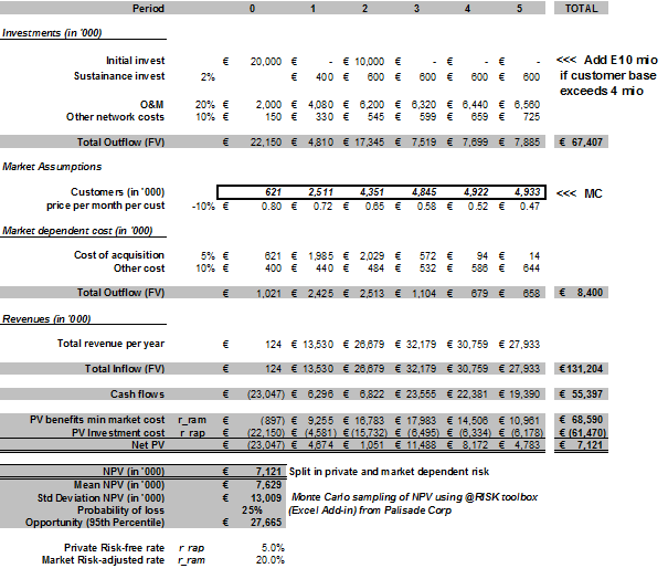
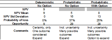
Obviously, if adding additional physical assets leads to verifiable incremental margin, then accepting incremental technology cost might be perfectly okay (let”s avoid being radical financial controllers).

Though its always wise to remember;

Cost committed is a certainty, incremental revenue is not.

NAUGHTY … IMAGINE A 5G MACRO CELLULAR NETWORK (OHH JE!).

From the NGMN whitepaper, it is clear that 5G is supposed to be served everywhere (albeit at very different quality levels) and not only in dense urban areas. Given the economical constraints (considered very lightly in the NGMN whitepaper) it is obvious that 5G would be available across operators existing macro-cellular networks and thus also in the existing macro cellular spectrum regime. Not that this gets a lot of attention.

In the following, I am proposing a 5G macro cellular overlay network providing a 1 Gbps persistent connection enabled by massive MiMo antenna systems. This though experiment is somewhat at odds with the NGMN whitepaper where their 50 Mbps promise might be more appropriate. Due to the relative high frequency range in this example, massive MiMo might still be practical as a deployment option.

If you follow all the 5G news, particular on 5G trials in US and Europe, you easily could get the impression that mm-wave frequencies (e.g., 30 GHz up-to 300 GHz) are the new black.

There is the notion that;

“Extremely high frequencies means extremely fast 5G speeds”

which is baloney! It is the extremely large bandwidth, readily available in the extremely high frequency bands, that make for extremely fast 5G (and LTE of course) speeds.

We can have GHz bandwidths instead of MHz (i.e, 1,000x) to play with! … How extremely cool is that not? We totally can suck at fundamental spectral efficiency and still get out extremely high throughputs for the consumers data consumption.

While this mm-wave frequency range is very cool, from an engineering perspective and for sure academically as well, it is also extremely non-matching our existing macro-cellular infrastructure with its 700 to 2.6 GHz working frequency range. Most mobile networks in Europe have been build on a 900 or 1800 MHz fundamental grid, with fill in from UMTS 2100 MHz coverage and capacity requirements.

Being a bit of a party pooper, I asked whether it wouldn’t be cool (maybe not to the extreme … but still) to deploy 5G as an overlay on our existing (macro) cellular network? Would it not be economically more relevant to boost the customer experience across our macro-cellular networks, that actually serves our customers today? As opposed to augment the existing LTE network with ultra hot zones of extreme speeds and possible also an extreme number of small cells.

If 5G would remain an above 3 GHz technology, it would be largely irrelevant to the mass market and most use cases.

A 5G MACRO CELLULAR THOUGHT EXAMPLE.

So let’s be (a bit) naughty and assume we can free up 20MHz @ 1800 MHz. After all, mobile operators tend to have a lot of this particular spectrum anyway. They might also re-purpose 3G/LTE 2.1 GHz spectrum (possibly easier than 1800 MHz pending overall LTE demand).

In the following, I am ignoring that whatever benefits I get out of deploying higher-order MiMo or massive MiMo (mMiMo) antenna systems, will work (almost) equally well for LTE as it will for 5G (all other things being equal).

Remember we are after

  • A lot more speed. At least 1 Gbps sustainable user throughput (in the downlink).
  • Ultra-responsiveness with latencies from 10 ms and down (E2E).
  • No worse 5G coverage than with LTE (at same frequency).

Of course if you happen to be a NGMN whitepaper purist, you will now tell me that I my ambition should only be to provide sustainable 50 Mbps per user connection. It is nevertheless an interesting thought exercise to explore whether residential areas could be served, by the existing macro cellular network, with a much higher consistent throughput than 50 Mbps that might ultimately be covered by LTE rather than needing to go to 5G. Anywhere both Rachid El Hattachi and Jarvan Erfenian knew well enough to hedge their 5G speed vision against the reality of economics and statistical fluctuation.

and I really don’t care about the 1,000x (LTE) bandwidth per unit area promise!

Why? The 1,000x promise It is fairly trivial promise. To achieve it, I simply need a high enough frequency and a large enough bandwidth (and those two as pointed out goes nicely hand in hand). Take a 100 meter 5G-cell range versus a 1 km LTE-cell range. The 5G-cell is 100 times smaller in coverage area and with 10x more 5G spectral bandwidth than for LTE (e.g., 200 MHz 5G vs 20 MHz LTE), I would have the factor 1,000 in throughput bandwidth per unit area. This without having to assume mMiMo that I could also choose to use for LTE with pretty much same effect.

Detour to the cool world of Academia: University of Bristol published recently (March 2016) a 5G spectral efficiency of ca. 80 Mbps/MHz in a 20 MHz channel. This is about 12 times higher than state of art LTE spectral efficiency. Their base station antenna system was based on so-called massive MiMo (mMiMo) with 128 antenna elements, supporting 12 users in the cell as approx. 1.6 Gbps (i.e., 20 MHz x 80 Mbps/MHz). The proof of concept system operated 3.5 GHz and in TDD mode (note: mMiMo does not scale as well for FDD and pose in general more challenges in terms of spectral efficiency). National Instruments provides a very nice overview of 5G MMiMo systems in their whitepaper “5G Massive MiMo Testbed: From Theory to Reality”.

A picture of the antenna system is shown below;

Figure above: One of the World’s First Real-Time massive MIMO Testbeds–Created at Lund University. Source: “5G Massive MiMo (mMiMo) Testbed: From Theory to Reality” (June 2016).

For a good read and background on advanced MiMo antenna systems I recommend Chockalingam & Sundar Rajan’s book on “Large MiMo Systems” (Cambridge University Press, 2014). Though there are many excellent accounts of simple MiMo, higher-order MiMo, massive MiMo, Multi-user MiMo antenna systems and the fundamentals thereof.

Back to naughty (i.e., my 5G macro cellular network);

So let’s just assume that the above mMiMO system, for our 5G macro-cellular network,

  • Ignoring that such systems originally were designed and works best for TDD based systems.
  • and keeping in mind that FDD mMiMo performance tends to be lower than TDD all else being equal.

will, in due time, be available for 5G with a channel of at least 20 MHz @ 1800MHz. And at a form factor that can be integrated well with existing macro cellular design without incremental TCO.

This is a very (VERY!) big assumption. Requirements of substantially more antenna space for massive MiMo systems, at normal cellular frequency ranges, are likely to result. Structural integrity of site designs would have to be checked and possibly be re-enforced to allow for the advanced antenna system, contributing to both additional capital cost and possible incremental tower/site lease.

So we have (in theory) a 5G macro-cellular overlay network with at least cell speeds of 1+Gbps, which is ca. 10 – 20 times that of today’s LTE networks cell performance (not utilizing massive MiMo!). If I have more 5G spectrum available, the performance would increase linearly (and a bit) accordingly.

The observant reader will know that I have largely ignored the following challenges of massive MiMo (see also Larsson et al’s “Massive MiMo for Next Generation Wireless Systems” 2014 paper);

  1. mMiMo designed for TDD, but works at some performance penalty for FDD.
  2. mMiMo will really be deployable at low total cost of ownership (i.e., it is not enough that the antenna system itself is low cost!).
  3. mMiMo performance leap frog comes at the price of high computational complexity (e.g., should be factored into the deployment cost).
  4. mMiMo relies on distributed processing algorithms which at this scale is relative un-exploited territory (i.e., should be factored into the deployment cost).

But wait a minute! I might (naively) theorize away additional operational cost of the active electronics and antenna systems on the 5G cell site (overlaid on legacy already present!). I might further assume that the Capex of the 5G radio & antenna system can be financed within the regular modernization budget (assuming such a budget exists). But … But surely our access and core transport networks have not been scaled for a factor 10 – 20 (and possibly a lot more than that) in crease in throughput per active customer?

No it has not! Really Not!

Though some modernized converged Telcos might be a lot better positioned for thefixed broadband transformation required to sustain the 5G speed promise.

For most mobile operators, it is highly likely that substantial re-design and investments of transport networks will have to be made in order to support the 5G target performance increase above and beyond LTE.

Definitely a lot more on this topic in a subsequent Blog.

ON THE 5G PROMISES.

Lets briefly examine the 8 above 5G promises or visionary statements and how these impact the underlying economics. As this is an introductory chapter, the deeper dive and analysis will be referred to subsequent chapters.

NEED FOR SPEED.

PROMISE 1: From 1 to 10 Gbps in actual experienced 5G speed per connected device (at a max. of 10 ms round-trip time).

PROMISE 2: Minimum of 50 Mbps per user connection everywhere (at a max. of 10 ms round-trip time).

PROMISE 3: Thousand times more bandwidth per unit area (compared to LTE).

Before anything else, it would be appropriate to ask a couple of questions;

“Do I need this speed?” (The expert answer if you are living inside the Telecom bubble is obvious! Yes Yes Yes ….Customer will not know they need it until they have it! …).

“that kind of sustainable speed for what?” (Telekom bubble answer would be! Lots of useful things! … much better video experience, 4K, 8K, 32K –> fully emerged holographic VR experience … Lots!)

“am I willing to pay extra for this vast improvement in my experience?” (Telekom bubble answer would be … ahem … that’s really a business model question and lets just have marketing deal with that later).

What is true however is:

My objective measurable 5G customer experience, assuming the speed-coverage-reliability promise is delivered, will quantum leap to un-imaginable levels (in terms of objectively measured performance increase).

Maybe more importantly, will the 5G customer experience from the very high speed and very low latency really be noticeable to the customer? (i.e, the subjective or perceived customer experience dimension).

Let’s ponder on this!

In Europe end of 2016, the urban LTE speed and latency user experience per connection would of course depend on which network the customer would be (not all being equal);

In 2016 on average in Europe an urban LTE user, experienced a DL speed of 31±9 Mbps, UL speed of 9±2 Mbps and latency around 41±9 milliseconds. Keep in mind that OpenSignal is likely to be closer to the real user’s smartphone OTT experience, as it pings a server external to the MNOs network. It should also be noted that although the OpenSignal measure might be closer to the real customer experience, it still does not provide the full experience from for example page load or video stream initialization and start.

The 31 Mbps urban LTE user experience throughput provides for a very good video streaming experience at 1080p (e.g., full high definition video) even on a large TV screen. Even a 4K video stream (15 – 32 Mbps) might work well, provided the connection stability is good and that you have the screen to appreciate the higher resolution (i.e., a lot bigger than your 5” iPhone 7 Plus). You are unlikely to see the slightest difference on your mobile device between the 1080p (9 Mbps) and 480p (1.0 – 2.3 Mbps) unless you are healthy young and/or with a high visual acuity which is usually reserved for the healthy & young.

With 5G, the DL speed is targeted to be at least 1 Gbps and could be as high as 10 Gbps, all delivered within a round trip delay of maximum 10 milliseconds.

5G target by launch (in 2020) is to deliver at least 30+ times more real experienced bandwidth (in the DL) compared to what an average LTE user would experience in Europe 2016. The end-2-end round trip delay, or responsiveness, of 5G is aimed to be at least 4 times better than the average experienced responsiveness of LTE in 2016. The actual experience gain between LTE and 3G has been between 5 – 10 times in DL speed, approx. 3 –5 times in UL and between 2 to 3 times in latency (i.e., pinging the same server exterior to the mobile network operator).

According with Sandvine’s 2015 report on “Global Internet Phenomena Report for APAC & Europe”, in Europe approx. 46% of the downstream fixed peak aggregate traffic comes from real-time entertainment services (e.g., video & audio streamed or buffered content such as Netflix, YouTube and IPTV in general). The same report also identifies that for Mobile (in Europe) approx. 36% of the mobile peak aggregate traffic comes from real-time entertainment. It is likely that the real share of real-time entertainment is higher, as video content embedded in social media might not be counted in the category but rather in Social Media. Particular for mobile, this would bring up the share with between 10% to 15% (more in line with what is actually measured inside mobile networks). Real-time entertainment and real-time services in general is the single most important and impacting traffic category for both fixed and mobile networks.

Video viewing experience … more throughput is maybe not better, more could be useless.

Video consumption is a very important component of real-time entertainment. It amounts to more than 90% of the bandwidth consumption in the category. The Table below provides an overview of video formats, number of pixels, and their network throughput requirements. The tabulated screen size is what is required (at a reasonable viewing distance) to detect the benefit of a given video format in comparison with the previous. So in order to really appreciate 4K UHD (ultra high definition) over 1080p FHD (full high definition), you would as a rule of thumb need double the screen size (note there are also other ways to improved the perceived viewing experience). Also for comparison, the Table below includes data for mobile devices, which obviously have a higher screen resolution in terms of pixels per inch (PPI) or dots per inch (DPI). Apart from 4K (~8 MP) and to some extend  8K (~33 MP), the 16K (~132 MP) and 32K (~528 MP) are still very yet exotic standards with limited mass market appeal (at least as of now).

We should keep in mind that there are limits to the human vision with the young and healthy having a substantial better visual acuity than what can be regarded as normal 20/20 vision. Most magazines are printed at 300 DPI and most modern smartphone displays seek to design for 300 DPI (or PPI) or more. Even Steve Jobs has addressed this topic;

However, it is fair to point out that  this assumed human vision limitation is debatable (and have been debated a lot). There is little consensus on this, maybe with the exception that the ultimate limit (at a distance of 4 inch or 10 cm) is 876 DPI or approx. 300 DPI (at 11.5 inch / 30 cm).

Anyway, what really matters is the customers experience and what they perceive while using their device (e.g., smartphone, tablet, laptop, TV, etc…).

So lets do the visual acuity math for smartphone like displays;

We see (from the above chart) that for an iPhone 6/7 Plus (5.5” display) any viewing distance above approx. 50 cm, a normal eye (i.e., 20/20 vision) would become insensitive to video formats better than 480p (1 – 2.3 Mbps). In my case, my typical viewing distance is ca. 30+ cm and I might get some benefits from 720p (2.3 – 4.5 Mbps) as opposed to 480p. Sadly my sight is worse than the norm of 20/20 (i.e., old! and let’s just leave it at that!) and thus I remain insensitive to the resolution improvements 720p would provide. If you have a device with at or below 4” display (e.g., iPhone 5 & 4) the viewing distance where normal eyes become insensitive is ca. 30+ cm.

All in all, it would appear that unless cellular user equipment, and the way these are being used, changes very fundamentally the 480p to 720p range might be more than sufficient.

If this is true, it also implies that a cellular 5G user on a reliable good network connection would need no more than 4 – 5 Mbps to get an optimum viewing (and streaming) experience (i.e., 720p resolution).

The 5 Mbps streaming speed, for optimal viewing experience, is very far away from our 5G 1-Gbps promise (x200 times less)!

Assuming instead of streaming we want to download movies, assuming we lots of memory available on our device … hmmm … then a typical 480p movie could be download in ca. 10 – 20 seconds at 1Gbps, a 720p movie between 30 and 40 seconds, and a 1080p would take 40 to 50 seconds (and likely a waste due to limitations to your vision).

However with a 5G promise of super reliable ubiquitous coverage, I really should not need to download and store content locally on storage that might be pretty limited.

Downloads to cellular devices or home storage media appears somewhat archaic. But would benefit from the promised 5G speeds.

I could share my 5G-Gbps with other users in my surrounding. A typical Western European household in 2020 (i.e., about the time when 5G will launch) would have 2.17 inhabitants (2.45 in Central Eastern Europe), watching individual / different real-time content would require multiples of the bandwidth of the optimum video resolution. I could have multiple video streams running in parallel, to likely the many display devices that will be present in the consumer’s home, etc… Still even at fairly high video streaming codecs, a consumer would be far away from consuming the 1-Gbps (imagine if it was 10 Gbps!).

Okay … so video consumption, independent of mobile or fixed devices, does not seem to warrant anywhere near the 1 – 10 Gbps per connection.

Surely EU Commission wants it!

EU Member States have their specific broadband coverage objectives – namely: ‘Universal Broadband Coverage with speeds at least 30 Mbps by 2020’ (i.e, will be met by LTE!) and ‘Broadband Coverage of 50% of households with speeds at least 100 Mbps by 2020 (also likely to be met with LTE and fixed broadband means’.

The European Commission’s “Broadband Coverage in Europe 2015” reports that 49.2% of EU28 Households (HH) have access to 100 Mbps (i.e., 50.8% of all HH have access to less than 100 Mbps) or more and 68.2% to broadband speeds above 30 Mbps (i.e., 32.8% of all HH with access to less than 30 Mbps). No more than 20.9% of HH within EU28 have FTTP (e.g., DE 6.6%, UK UK 1.4%, FR 15.5%, DK 57%).

The EU28 average is pretty good and in line with the target. However, on an individual member state level, there are big differences. Also within each of the EU member states great geographic variation is observed in broadband coverage.

Interesting, the 5G promises to per user connection speed (1 – 10 Gbps), coverage (user perceived 100%) and reliability (user perceived 100%) is far more ambitious that the broadband coverage objectives of the EU member states.

So maybe indeed we could make the EU Commission and Member States happy with the 5G Throughput promise. (this point should not be underestimated).

Web browsing experience … more throughput and all will be okay myth!

So … Surely, the Gbps speeds can help provide a much faster web browsing / surfing experience than what is experienced today for LTE and for the fixed broadband? (if there ever was a real Myth!).

In other words the higher the bandwidth, the better the user’s web surfing experience should become.

While bandwidth (of course) is a factor in customers browsing experience, it is but a factor out of several that also governs the customers real & perceived internet experience; e.g., DNS Lookups (this can really mess up user experience), TCP, SSL/TLS negotiation, HTTP(S) requests, VPN, RTT/Latency, etc…

An excellent account of these various effects is given by Jim Getty’s “Traditional AQM is not enough” (i.e., AQM: Active Queue Management). Measurements (see Jim Getty’s blog) strongly indicates that at a given relative modest bandwidth (>6+ Mbps) there is no longer any noticeable difference in page load time. In my opinion there are a lot of low hanging fruits in network optimization that provides large relative improvements in customer experience than network speed alone..

Thus one might carefully conclude that, above a given throughput threshold it is unlikely that more throughput would have a significant effect on the consumers browsing experience.

More work needs to be done in order to better understand the experience threshold after which more connection bandwidth has diminishing returns on the customer’s browsing experience. However, it would appear that 1-Gbps 5G connection speed would be far above that threshold. An average web page in 2016 was 2.2 MB which from an LTE speed perspective would take 568 ms to load fully provided connection speed was the only limitation (which is not the case). For 5G the same page would download within 18 ms assuming that connection speed was the only limitation.

Downloading content (e.g., FTTP). 

Now we surely are talking. If I wanted to download the whole Library of the US Congress (I like digital books!), I am surely in need for speed!?

The US Congress have estimated that the whole print collection (i.e., 26 million books) adds up to 208 terabytes.Thus assuming I have 208+ TB of storage, I could within 20+ (at 1 Gbps) to 2+ (at 20 Gbps) days download the complete library of the US Congress.

In fact, at 1 Gbps would allow me to download 15+ books per second (assuming 1 book is on average 3oo pages and formatted at 600 DPI TIFF which is equivalent to ca. 8 Mega Byte).

So clearly, for massive file sharing (music, videos, games, books, documents, etc…), the 5G speed promise is pretty cool.

Though, it does assume that consumers would continue to see a value in storing information locally on their personally devices or storage medias. The idea remains archaic, but I guess there will always be renaissance folks around.

What about 50 Mbps everywhere (at a 10 ms latency level)?

Firstly, providing a customers with a maximum latency of 10 ms with LTE is extremely challenging. It would be highly unlikely to be achieved within existing LTE networks, particular if transmission retrials are considered. From OpenSignal December 2016 measurements shown in the chart below, for urban areas across Europe, the LTE latency is on average around 41±9 milliseconds. Considering the LTE latency variation we are still 3 – 4 times away from the 5G promise. The country average would be higher than this. Clearly this is one of the reasons why the NGMN whitepaper proposes a new air-interface. As well as some heavy optimization and redesigns in general across our Telco networks.

The urban LTE persistent experience level is very reasonable but remains lower than the 5G promise of 50 Mbps, as can be seen from the chart below;

The LTE challenge however is not the customer experience level in urban areas but on average across a given geography or country. Here LTE performs substantially worse (also on throughput) than what the NGMN whitepaper’s ambition is. Let us have a look at the current LTE experience level in terms of LTE coverage and in terms of (average) speed.

Based on European Commission “Broadband Coverage in Europe 2015” we observe that on average the total LTE household coverage is pretty good on an EU28 level. However, the rural households are in general underserved with LTE. Many of the EU28 countries still lack LTE consistent coverage in rural areas. As lower frequencies (e.g., 700 – 900 MHz) becomes available and can be overlaid on the existing rural networks, often based on 900 MHz grid, LTE rural coverage can be improved greatly. This economically should be synchronized with the normal modernization cycles. However, with the current state of LTE (and rural network deployments) it might be challenging to reach a persistent level of 50 Mbps per connection everywhere. Furthermore, the maximum 10 millisecond latency target is highly unlikely to be feasible with LTE.

In my opinion, 5G would be important in order to uplift the persistent throughput experience to at least 50 Mbps everywhere (including cell edge). A target that would be very challenging to reach with LTE in the network topologies deployed in most countries (i.e., particular outside urban/dense urban areas).

The customer experience value to the general consumer of a maximum 10 millisecond latency is in my opinion difficult to assess. At a 20 ms response time would most experiences appear instantaneous. The LTE performance of ca. 40 ms E2E external server response time, should satisfy most customer experience use case requirements beside maybe VR/AR.

Nevertheless, if the 10 ms 5G latency target can be designed into the 5G standard without negative economical consequences then that might be very fine as well.

Another aspect that should be considered is the additional 5G market potential of providing a persistent 50 Mbps service (at a good enough & low variance latency). Approximately 70% of EU28 households have at least a 30 Mbps broadband speed coverage. If we look at EU28 households with at least 50 Mbps that drops to around 55% household coverage. With the 100% (perceived)coverage & reliability target of 5G as well as 50 Mbps everywhere, one might ponder the 30% to 45% potential of households that are likely underserved in term of reliable good quality broadband. Pending the economics, 5G might be able to deliver good enough service at a substantial lower cost compared more fixed centric means.

Finally, following our expose on video streaming quality, clearly a 50 Mbps persistent 5G connectivity would be more than sufficient to deliver a good viewing experience. Latency would be less of an issue in the viewing experience as longs as the variation in the latency can be kept reasonable low.


Acknowledgement

I greatly acknowledge my wife Eva Varadi for her support, patience and understanding during the creative process of creating this Blog.


WORTHY 5G & RELATED READS.

  1. “NGMN 5G White Paper” by R.El Hattachi & J. Erfanian (NGMN Alliance, February 2015).
  2. “Understanding 5G: Perspectives on future technological advancement in mobile” by D. Warran & C. Dewar (GSMA Intelligence December 2014).
  3. “Fundamentals of 5G Mobile Networks” by J. Rodriguez (Wiley 2015).
  4.  “The 5G Myth: And why consistent connectivity is a better future” by William Webb (2016).
  5. “Software Networks: Virtualization, SDN, 5G and Security”by G. Pujolle (Wile 2015).
  6. “Large MiMo Systems” by A. Chockalingam & B. Sundar Rajan (Cambridge University Press 2014).
  7. “Millimeter Wave Wireless Communications” by T.S. Rappaport, R.W. Heath Jr., R.C. Daniels, J.N. Murdock (Prentis Hall 2015).
  8. “The Limits of Human Vision” by Michael F. Deering (Sun Microsystems).
  9. “Quad HD vs 1080p vs 720p comparison: here’s what’s the difference” by Victor H. (May 2014).
  10. “Broadband Coverage in Europe 2015: Mapping progress towards the coverage objectives of the Digital Agenda” by European Commission, DG Communications Networks, Content and Technology (2016).

The Unbearable Lightness of Mobile Voice.

Advertisements
  • Mobile data adaption can be (and usually is) very un-healthy for the mobile voice revenues.
  • A Mega Byte of Mobile Voice is 6 times more expensive than a Mega Byte of Mobile Data (i.e., global average) 
  • If customers would pay the Mobile Data Price for Mobile Voice, 50% of Global Mobile Revenue would Evaporate (based on 2013 data).
  • Classical Mobile Voice is not Dead! Global Mobile Voice Usage grew with more than 50% over the last 5 years. Though Global Voice Revenue remained largely constant (over 2009 – 2013). 
  • Mobile Voice Revenues declined in most Western European & Central Eastern European countries.
  • Voice Revenue in Emerging Mobile-Data Markets (i.e., Latin America, Africa and APAC) showed positive growth although decelerating.
  • Mobile Applications providing high-quality (often High Definition) mobile Voice over IP should be expected to dent the classical mobile voice revenues (as Apps have impacted SMS usage & revenue).
  • Most Western & Central Eastern European markets shows an increasing decline in price elasticity of mobile voice demand. Even some markets (regions) had their voice demand decline as the voice prices were reduced (note: not that causality should be deduced from this trend though).
  • The Art of Re-balancing (or re-capture) the mobile voice revenue in data-centric price plans are non-trivial and prone to trial-and-error (but likely also un-avoidable).

An Unbearable Lightness.

There is something almost perverse about how light the mobile industry tends to treat Mobile Voice, an unbearable lightness?

How often don’t we hear Telco Executives wish for All-IP and web-centric services for All? More and more mobile data-centric plans are being offered with voice as an after thought. Even though voice still constitute more than 60% of the Global Mobile turnover  and in many emerging mobile markets beyond that. Even though classical mobile voice is more profitable than true mobile broadband access. “Has the train left the station” for Voice and running off the track? In my opinion, it might have for some Telecom Operators, but surely not for all. Taking some time away from thinking about mobile data would already be an incredible improvement if spend on strategizing and safeguarding mobile voice revenues that still are a very substantial part of The Mobile Business Model.

Mobile data penetration is un-healthy for voice revenue. It is almost guarantied that voice revenue will start declining as the mobile data penetration reaches 20% and beyond. There are very few exceptions (i.e., Australia, Singapore, Hong Kong and Saudi Arabia) to this rule as observed in the figure below. Much of this can be explained by the Telecoms focus on mobile data and mobile data centric strategies that takes the mobile voice business for given or an afterthought … focusing on a future of All-IP Services where voice is “just” another data service. Given the importance of voice revenues to the mobile business model, treating voice as an afterthought is maybe not the most value-driven strategy to adopt.

I should maybe point out that this is not per se a result of the underlying Cellular All-IP Technology. The fact is that Cellular Voice over an All-IP network is very well specified within 3GPP. Voice over LTE (i.e., VoLTE), or Voice over HSPA (VoHSPA) for that matter, is enabled with the IP Multimedia Subsystem (IMS). Both VoLTE and VoHSPA, or simply Cellular Voice over IP (Cellular VoIP as specified by 3GPP), are highly spectral efficient (compared to their circuit switched equivalents). Further the Cellular VoIP can be delivered at a high quality comparable to or better than High Definition (HD) circuit switched voice. Recent Mean Opinion Score (MOS) measurements by Ericsson and more recently (August 2014) Signals Research Group & Spirent have together done very extensive VoLTE network benchmark tests including VoLTE comparison with the voice quality of 2G & 3G Voice as well as Skype (“Behind the VoLTE Curtain, Part 1. Quantifying the Performance of a Commercial VoLTE Deployment”). Further advantage of Cellular VoIP is that it is specified to inter-operate with legacy circuit-switched networks via the circuit-switched fallback functionality. An excellent account for Cellular VoIP and VoLTE in particular can be found in Miikki Poikselka  et al’s great book on “Voice over LTE” (Wiley, 2012).

Its not the All-IP Technology that is wrong, its the commercial & strategic thinking of Voice in an All-IP World that leaves a lot to be wished for.

Voice over LTE provides for much better Voice Quality than a non-operator controlled (i.e., OTT) mobile VoIP Application would be able to offer. But is that Quality worth 5 to 6 times the price of data, that is the Billion $ Question.

  • Figure Above: illustrates the compound annual growth rates (2009 to 2013) of mobile voice revenue and the mobile data penetration at the beginning of the period (i.e., 2009). As will be addressed later it should be noted that the growth of mobile voice revenues are NOT only depending on Mobile Data Penetration Rates but on a few other important factors, such as addition of new unique subscribers, the minute price and the voice arpu compared to the income level (to name a few). Analysis has been based on Pyramid Research data. Abbreviations: WEU: Western Europe, CEE: Central Eastern Europe, APAC: Asia Pacific, MEA: Middle East & Africa, NA: North America and LA: Latin America.

In the following discussion classical mobile voice should be understood as an operator-controlled voice service charged by the minute or in equivalent economical terms (i.e., re-balanced data pricing). This is opposed to a mobile-application-based voice service (outside the direct control of the Telecom Operator) charged by the tariff structure of a mobile data package without imposed re-balancing.

If the Industry would charge a Mobile Voice Minute the equivalent of what they charge a Mobile Mega Byte … almost 50% of Mobile Turnover would disappear … So be careful AND be prepared for what you wish for! 

There are at least a couple of good reasons why Mobile Operators should be very focused on preserving mobile voice as we know it (or approximately so) also in LTE (and any future standards). Even more so, Mobile Operators should try to avoid too many associations with non-operator controlled Voice-over-IP (VoIP) Smartphone applications (easier said than done .. I know). It will be very important to define a future voice service on the All-IP Mobile Network that maintains its economics (i.e., pricing & margin) and don’t get “confused” with the mobile-data-based economics with substantially lower unit prices & questionable profitability.

Back in 2011 at the Mobile Open Summit, I presented “Who pays for Mobile Broadband” (i.e., both in London & San Francisco) with the following picture drawing attention to some of the Legacy Service (e.g., voice & SMS) challenges our Industry would be facing in the years to come from the many mobile applications developed and in development;

One of the questions back in 2011 was (and Wow it still is! …) how to maintain the Mobile ARPU & Revenues at a reasonable level, as opposed to massive loss of revenue and business model sustainability that the mobile data business model appeared to promise (and pretty much still does). Particular the threat (& opportunities) from mobile Smartphone applications. Mobile Apps that provides Mobile Customers with attractive price-arbitrage compared to their legacy prices for SMS and Classical Voice.

IP killed the SMS Star” … Will IP also do away with the Classical Mobile Voice Economics as well?

Okay … Lets just be clear about what is killing SMS (it’s hardly dead yet). The Mobile Smartphone  Messaging-over-IP (MoIP) App does the killing. However, the tariff structure of an SMS vis-a-vis that of a mobile Mega Byte (i..e, ca. 3,000x) is the real instigator of the deed together with the shear convenience of the mobile application itself.

As of August 2014 the top Messaging & Voice over IP Smartphone applications share ca. 2.0+ Billion Active Users (not counting Facebook Messenger and of course with overlap, i.e., active users having several apps on their device). WhatsApp is the Number One Mobile Communications App with about 700 Million active users  (i.e., up from 600 Million active users in August 2014). Other Smartphone Apps are further away from the WhatsApp adaption figures. Applications from Viber can boast of 200+M active users, WeChat (predominantly popular in Asia) reportedly have 460+M active users and good old Skype around 300+M active users. The impact of smartphone MoIP applications on classical messaging (e.g., SMS) is well evidenced. So far Mobile Voice-over-IP has not visible dented the Telecom Industry’s mobile voice revenues. However the historical evidence is obviously no guaranty that it will not become an issue in the future (near, medium or far).

WhatsApp is rumoured to launch mobile voice calling as of first Quarter of 2015 … Will this event be the undoing of operator controlled classical mobile voice?  WhatsApp already has taken the SMS Scalp with 30 Billion WhatsApp messages send per day according the latest data from WhatsApp (January 2015). For comparison the amount of SMS send out over mobile networks globally was a bit more than 20 Billion per day (source: Pyramid Research data). It will be very interesting (and likely scary as well) to follow how WhatsApp Voice (over IP) service will impact Telecom operator’s mobile voice usage and of course their voice revenues. The Industry appears to take the news lightly and supposedly are unconcerned about the prospects of WhatsApp launching a mobile voice services (see: “WhatsApp voice calling – nightmare for mobile operators?” from 7 January 2015) … My favourite lightness is Vodacom’s (South Africa) “if anything, this vindicates the massive investments that we’ve been making in our network….” … Talking about unbearable lightness of mobile voice … (i.e., 68% of the mobile internet users in South Africa has WhatsApp on their smartphone).

Paying the price of a mega byte mobile voice.

A Mega-Byte is not just a Mega-Byte … it is much more than that!

In 2013, the going Global average rate of a Mobile (Data) Mega Byte was approximately 5 US-Dollar Cent (or a Nickel). A Mega Byte (MB) of circuit switched voice (i.e., ca. 11 Minutes @ 12.2kbps codec) would cost you 30+ US$-cent or about 6 times that of Mobile Data MB. Would you try to send a MB of SMS (i.e., ca. 7,143 of them) that would cost you roughly 150 US$ (NOTE: US$ not US$-Cents).

1 Mobile MB = 5 US$-cent Data MB < 30+ US$-cent Voice MB (6x mobile data) << 150 US$ SMS MB (3000x mobile data).

A Mega Byte of voice conversation is pretty un-ambiguous in the sense of being 11 minutes of a voice conversation (typically a dialogue, but could be monologue as well, e.g., voice mail or an angry better half) at a 12.2 kbps speech codec. How much mega byte a given voice conversation will translate into will depend on the underlying speech coding & decoding  (codec) information rate, which typically is 12.2 kbps or 5.9 kbps (i.e., for 3GPP cellular-based voice). In general we would not be directly conscious about speed (e.g., 12.2 kbps) at which our conversation is being coded and decoded although we certainly would be aware of the quality of the codec itself and its ability to correct errors that will occur in-between the two terminals. For a voice conversation itself, the parties that engage in the conversation is pretty much determining the duration of the conversation.

An SMS is pretty straightforward and well defined as well, i.e., being 140 Bytes (or characters). Again the underlying delivery speed is less important as for most purposes it feels that the SMS sending & delivery is almost instantaneously (though the reply might not be).

All good … but what about a Mobile Data Byte? As a concept it could by anything or nothing. A Mega Byte of Data is Extremely Ambiguous. Certainly we get pretty upset if we perceive a mobile data connection to be slow. But the content, represented by the Byte, would obviously impact our perception of time and whether we are getting what we believe we are paying for. We are no longer master of time. The Technology has taken over time.

Some examples: A Mega Byte of Voice is 11 minutes of conversation (@ 12.2 kbps). A Mega Byte of Text might take a second to download (@ 1 Mbps) but 8 hours to process (i.e., read). A Mega Byte of SMS might be delivered (individually & hopefully for you and your sanity spread out over time) almost instantaneously and would take almost 16 hours to read through (assuming English language and an average mature reader). A Mega Byte of graphic content (e.g., a picture) might take a second to download and milliseconds to process. Is a Mega Byte (MB) of streaming music that last for 11 seconds (@ 96 kbps) of similar value to a MB of Voice conversation that last for 11 minutes or a MB millisecond picture (that took a second to download).

In my opinion the answer should be clearly NO … Such (somewhat silly) comparisons serves to show the problem with pricing and valuing a Mega Byte. It also illustrates the danger of ambiguity of mobile data and why an operator should try to avoid bundling everything under the banner of mobile data (or at the very least be smart about it … whatever that means).

I am being a bit naughty in above comparisons, as I am freely mixing up the time scales of delivering a Byte and the time scales of neurological processing that Byte (mea culpa).


  • Figure Above: Logarithmic representation of the cost per Mega Byte of a given mobile service. 1 MB of Voice is roughly corresponding to 11 Minutes at a 12.2 voice codec which is ca. 25+ times the monthly global MoU usage. 1 MB of SMS correspond to ca. 7,143 SMSs which is a lot (actually really a lot). In USA 7,143 would roughly correspond to a full years consumption. However, in WEU 7,143 SMS would be ca. 6+ years of SMS consumption (on average) to about almost 12 years of SMS consumption in MEA Region. Still SMS remain proportionate costly and clear is an obvious service to be rapidly replaced by mobile data as it becomes readily available. Source: Pyramid Research.

The “Black” Art of Re-balancing … Making the Lightness more Bearable?

I recently had a discussion with a very good friend (from an emerging market) about how to recover lost mobile voice revenues in the mobile data plans (i.e., the art of re-balancing or re-capturing). Could we do without Voice Plans? Should we focus on All-in the Data Package? Obviously, if you would charge 30+ US$-cent per Mega Byte Voice, while you charge 5 US$-cent for Mobile Data, that might not go down well with your customers (or consumer interest groups). We all know that “window-dressing” and sleight-of-hand are important principles in presenting attractive pricings. So instead of Mega Byte voice we might charge per Kilo Byte (lower numeric price), i.e., 0.029 US$-cent per kilo byte (note: 1 kilo-byte is ca. 0.65 seconds @ 12.2 kbps codec). But in general the consumer are smarter than that. Probably the best is to maintain a per time-unit charge or to Blend in the voice usage & pricing into the Mega Byte Data Price Plan (and hope you have done your math right).

Example (a very simple one): Say you have 500 MB mobile data price plan at 5 US$-cent per MB (i.e., 25 US$). You also have a 300 Minute Mobile Voice Plan of 2.7 US$-cent a minute (or 30 US$-cent per MB). Now 300 Minutes corresponds roughly to 30 MB of Voice Usage and would be charged ca. 9$. Instead of having a Data & Voice Plan, one might have only the Data Plan charging (500 MB x 5 US$cent/MB + 30 MB x 30 US$/cent/MB) / 530 MB or 6.4 US$-cent per MB (or 1.4 US$-cent more for mobile voice over the data plan or a 30% surcharge for Voice on the Mobile Data Bytes). Obviously such a pricing strategy (while simple) does pose some price strategic challenges and certainly does not per se completely safeguard voice revenue erosion. Keeping Mobile Voice separately from Mobile Data (i.e., Minutes vs Mega Bytes) in my opinion will remain the better strategy. Although such a minutes-based strategy is easily disrupted by innovative VoIP applications and data-only entrepreneurs (as well as Regulator Authorities).

Re-balancing (or re-capture) the voice revenue in data-centric price plans are non-trivial and prone to trial-and-error. Nevertheless it is clearly an important pricing strategy area to focus on in order to defend existing mobile voice revenues from evaporating or devaluing by the mobile data price plan association.

Is Voice-based communication for the Masses (as opposed to SME, SOHO, B2B,Niche demand, …) technologically un-interesting? As a techno-economist I would say far from it. From the GSM to HSPA and towards LTE, we have observed a quantum leap, a factor 10, in voice spectral efficiency (or capacity), substantial boost in link-budget (i.e., approximately 30% more geographical area can be covered with UMTS as opposed to GSM in apples for apples configurations) and of course increased quality (i.e., high-definition or crystal clear mobile voice). The below Figure illustrates the progress in voice capacity as a function of mobile technology. The relative voice spectral efficiency data in the below figure has been derived from one of the best (imo) textbooks on mobile voice “Voice over LTE” by Miikki Poikselka et all (Wiley, 2012);

  • Figure Above: Abbreviation guide;  EFR: Enhanced Full Rate, AMR: Adaptive Multi-Rate, DFCA: Dynamic Frequency & Channel Allocation, IC: Interference Cancellation. What might not always be appreciate is the possibility of defining voice over HSPA, similar to Voice over LTE. Source: “Voice over LTE” by Miikki Poikselka et all (Wiley, 2012).

If you do a Google Search on Mobile Voice you would get ca. 500 Million results (note Voice over IP only yields 100+ million results). Try that on Mobile Data and “sham bam thank you mam” you get 2+ Billion results (and projected to increase further). For most of us working in the Telecom industry we spend very little time on voice issues and an over-proportionate amount of time on broadband data. When you tell your Marketing Department that a state-of-the-art 3G can carry at least twice as much voice traffic than state-of-the –art GSM (and over 30% more coverage area) they don’t really seem to get terribly exited? Voice is un-sexy!? an afterthought!? … (don’t even go brave and tell Marketing about Voice over LTE, aka VoLTE).

Is Mobile Voice Dead or at the very least Dying?

Is Voice un-interesting, something to be taken for granted?

Is Voice “just” data and should be regarded as an add-on to Mobile Data Services and Propositions?

From a Mobile Revenue perspective mobile voice is certainly not something to be taken for granted or just an afterthought. In 2013, mobile voice still amounted for 60+% of he total global mobile turnover, with mobile data taking up ca. 40% and SMS ca. 10%. There are a lot of evidence that SMS is dying out quickly with the emergence of smartphones and Messaging-over-IP-based mobile application (SMS – Assimilation is inevitable, Resistance is Futile!). Not particular surprising given the pricing of SMS and the many very attractive IP-based alternatives. So are there similar evidences of mobile voice dying?

NO! NIET! NEM! MA HO BU! NEJ! (not any time soon at least)

Lets see what the data have to say about mobile voice?

In the following I only provide a Regional but should there be interest I have very detailed deep dives for most major countries in the various regions. In general there are bigger variations to the regional averages in Middle East & Africa (i.e., MEA) as well as Asia Pacific (i.e., APAC) Regions, as there is a larger mix of mature and emerging markets with fairly large differences in mobile penetration rates and mobile data adaptation in general. Western Europe, Central Eastern Europe, North America (i.e., USA & Canada) and Latin America are more uniform in conclusions that can reasonably be inferred from the averages.

As shown in the Figure below, from 2009 to 2013, the total amount of mobile minutes generated globally increased with 50+%. Most of that increase came from emerging markets as more share of the population (in terms of individual subscribers rather than subscriptions) adapted mobile telephony. In absolute terms, the global mobile voice revenues did show evidence of stagnation and trending towards decline.


  • Figure Above: Illustrates the development & composition of historical Global Mobile Revenues over the period 2009 to 2013. In addition also shows the total estimated growth of mobile voice minutes (i.e., Red Solid Curve showing MoUs in units of Trillions) over the period. Sources: Pyramid Research & Statista. It should noted that various data sources actual numbers (over the period) are note completely matching. I have observed a difference between various sources of up-to 15% in actual global values. While interesting this difference does not alter the analysis & conclusions presented here.

If all voice minutes was charged with the current Rate of Mobile Data, approximately Half-a-Billion US$ would evaporate from the Global Mobile Revenues.

So while mobile voice revenues might not be a positive growth story its still “sort-of” important to the mobile industry business.

Most countries in Western & Central Eastern Europe as well as mature markets in Middle East and Asia Pacific shows mobile voice revenue decline (in absolute terms and in their local currencies). For Latin America, Africa and Emerging Mobile Data Markets in Asia-Pacific almost all exhibits positive mobile voice revenue growth (although most have decelerating growth rates).

  • Figure Above: Illustrates the annual growth rates (compounded) of total mobile voice revenues and the corresponding growth in mobile voice traffic (i.e., associated with the revenues). Some care should be taken as for each region US$ has been used as a common currency. In general each individual country within a region has been analysed based on its own local currency in order to avoid mixing up currency exchange effects. Source: Pyramid Research.

Of course revenue growth of the voice service will depend on (1) the growth of subscriber base, (2) the growth of the unit itself (i.e., minutes of voice usage) as it is used by the subscribers (i.e., which is likely influenced by the unit price), and (3) the development of the average voice revenue per subscriber (or user) or the unit price of the voice service. Whether positive or negative growth of Revenue results, pretty much depends on the competitive environment, regulatory environment and how smart the business is in developing its pricing strategy & customer acquisition & churn dynamics.

Growth of (unique) mobile customers obviously depends the level of penetration, network coverage & customer affordability. Growth in highly penetrated markets is in general (much) lower than growth in less mature markets.

  • Figure Above: Illustrates the annual growth rates (compounded) of unique subscribers added to a given market (or region). Further to illustrate the possible relationship between increased subscribers and increased total generated mobile minutes the previous total minutes annual growth is shown as well. Source: Pyramid Research.

Interestingly, particular for the North America Region (NA), we see an increase in unique subscribers of 11% per anno and hardly any growth over the  period of total voice minutes. Firstly, note that the US Market will dominate the averaging of the North America Region (i.e., USA and Canada) having approx. 13 times more subscribers. So one of the reasons for this no-minutes-growth effect is that the US market saw a substantial increase in the prepaid ratio (i.e., from ca.19% in 2009 to 28% in 2013). Not only were new (unique) prepaid customers being added. Also a fairly large postpaid to prepaid migration took place over the period. In the USA the minute usage of a prepaid is ca. 35+% lower than that of a postpaid. In comparison the Global demanded minutes difference is 2.2+ times lower prepaid minute usage compared to that of a postpaid subscriber). In the NA Region (and of course likewise in the USA Market) we observe a reduced voice usage over the period both for the postpaid & prepaid segment (based on unique subscribers). Thus increased prepaid blend in the overall mobile base with a relative lower voice usage combined with a general decline in voice usage leads to a pretty much zero growth in voice usage in the NA Market. Although the NA Region is dominated by USA growth (ca. 0.1 % CAGR total voice growth), Canada’s likewise showed very minor growth in their overall voice usage as well (ca. 3.8% CAGR). Both Canada & USA reduced their minute pricing over the period.

  • Note on US Voice Usage & Revenues: note that in both in US and in Canada also the receiving party pays (RPP) for receiving a voice call. Thus revenue generating minutes arises from both outgoing and incoming minutes. This is different from most other markets where the Calling Party Pays (CPP) and only minutes originating are counted in the revenue generation. For example in USA the Minutes of Use per blended customer was ca. 620 MoU in 2013. To make that number comparable with say Europe’s 180 MoU, one would need to half the US figure to 310 MoU still a lot higher than the Western European blended minutes of use. The US bundles are huge (in terms of allowed minutes) and likewise the charges outside bundles (i.e., forcing the consumer into the next one) though the fixed fees tends be high to very high (in comparison with other mobile markets). The traditional US voice plan would offer unlimited on-net usage (i.e., both calling & receiving party are subscribing to the same mobile network operator) as well as unlimited off-peak usage (i.e., evening/night/weekends). It should be noted that many new US-based mobile price plans offers data bundles with unlimited voice (i.e., data-centric price plans). In 2013 approximately 60% of the US mobile industry’s turnover could be attributed to mobile voice usage. This number is likely somewhat higher as some data-tariffs has voice-usage (e.g., typically unlimited) embedded. In particular the US mobile voice business model would be depending customer migration to prepaid or lower-cost bundles as well as how well the voice-usage is being re-balanced (and re-captured) in the Data-centric price plans.

The second main component of the voice revenue is the unit price of a voice minute. Apart from the NA Region, all markets show substantial reductions in the unit price of a minute.

  • Figure Above: Illustrating the annual growth (compounded) of the per minute price in US$-cents as well as the corresponding growth in total voice minutes. The most affected by declining growth is Western Europe & Central Eastern Europe although other more-emerging markets are observed to have decelerating voice revenue growth. Source: Pyramid Research.

Clearly from the above it appears that the voice “elastic” have broken down in most mature markets with diminishing (or no return) on further minute price reductions. Another way of looking at the loss (or lack) of voice elasticity is to look at the unit-price development of a voice-minute versus the growth of the total voice revenues;

  • Figure Above: Illustrates the growth of Total Voice Revenue and the unit-price development of a mobile voice minute. Apart from the Latin America (LA) and Asia Pacific (APAC) markets there clearly is no much further point in reducing the price of voice. Obviously, there are other sources & causes, than the pure gain of elasticity, effecting the price development of a mobile voice minute (i.e., regulatory, competition, reduced demand/voice substitution, etc..). Note US$ has been used as the unifying currency across the various markets. Despite currency effects the trend is consistent across the markets shown above. Source: Pyramid Research.

While Western & Central-Eastern Europe (WEU & CEE) as well as the mature markets in Middle East and Asia-Pacific shows little economic gain in lowering voice price, in the more emerging markets (LA and Africa) there are still net voice revenue gains to be made by lowering the unit price of a minute (although the gains are diminishing rapidly). Although most of the voice growth in the emerging markets comes from adding new customers rather than from growth in the demand per customer itself.

  • Figure Above: Illustrating possible drivers for mobile voice growth (positive as well as negative); such as Mobile Data Penetration 2013 (expected negative growth impact), increased number of (unique) subscribers compared to 2009 (expected positive growth impact) and changes in prepaid-postpaid blend (a negative %tage means postpaid increased their proportion while a positive %tage translates into a higher proportion of prepaid compared to 2009). Voice tariff changes have been observed to have elastic effects on usage as well although the impact changes from market to market pending on maturity. Source: derived from Pyramid Research.

With all the talk about Mobile Data, it might come as a surprise that Voice Usage is actually growing across all regions with the exception of North America. The sources of the Mobile Voice Minutes Growth are largely coming from

  1. Adding new unique subscribers (i.e., increasing mobile penetration rates).
  2. Transitioning existing subscribers from prepaid to postpaid subscriptions (i.e., postpaid tends to have (a lot) higher voice usage compared to prepaid).
  3. General increase in usage per individual subscriber (i.e., few markets where this is actually observed irrespective of the general decline in the unit cost of a voice minute).

To the last point (#3) it should be noted that the general trend across almost all markets is that Minutes of Use per Unique customer is stagnating and even in decline despite substantial per unit price reduction of a consumed minute. In some markets that trend is somewhat compensated by increase of postpaid penetration rates (i.e., postpaid subscribers tend to consume more voice minutes). The reduction of MoUs per individual subscriber is more significant than a subscription-based analysis would let on.

Clearly, Mobile Voice Usage is far from Dead

and

Mobile Voice Revenue is a very important part of the overall mobile revenue composition.

It might make very good sense to spend a bit more time on strategizing voice, than appears to be the case today. If mobile voice remains just an afterthought of mobile data, the Telecom industry will loose massive amounts of Revenues and last but not least Profitability.


Post Script: What drives the voice minute growth?

An interesting exercise is to take all the data and run some statistical analysis on it to see what comes out in terms of main drivers for voice minute growth, positive as well as negative. The data available to me comprises 77 countries from WEU (16), CEE (8), APAC (15), MEA (17), NA (Canada & USA) and LA (19). I am furthermore working with 18 different growth parameters (e.g., mobile penetration, prepaid share of base, data adaptation, data penetration begin of period, minutes of use, voice arpu, voice minute price, total minute volume, customers, total revenue growth, sms, sms price, pricing & arpu relative to nominal gdp etc…) and 7 dummy parameters (populated with noise and unrelated data).

Two specific voice minute growth models emerges our of a comprehensive analysis of the above described data. The first model is as follows

(1) Voice Growth correlates positively with Mobile Penetration (of unique customers) in the sense of higher penetration results in more minutes, it correlates negatively with Mobile Data Penetration at the begin of the period (i.e., 2009 uptake of 3G, LTE and beyond) in the sense that higher mobile data uptake at the begin of the period leads to a reduction of Voice Growth, and finally  Voice Growth correlates negatively with the Price of a Voice Minute in the sense of higher prices leads to lower growth and lower prices leads to higher growth.  This model is statistically fairly robust (e.g., a p-values < 0.0001) as well as having all parameters with a statistically meaningful confidence intervals (i.e., upper & lower 95% confidence interval having the same sign).

The Global Analysis does pin point to very rational drivers for mobile voice usage growth, i.e., that mobile penetration growth, mobile data uptake and price of a voice minute are important drivers for total voice usage. 

It should be noted that changes in the prepaid proportion does not appear statistically to impact voice minute growth.

The second model provides a marginal better overall fit to the Global Data but yields slightly worse p-values for the individual descriptive parameters.

(2) The second model simply adds the Voice ARPU to (nominal) GDP ratio to the first model. This yields a negative correlation in the sense that a low ratio results in higher voice usage growth and a higher ration in lower voice usage growth.

Both models describe the trends or voice growth dynamics reasonably well, although less convincing for Western & Central Eastern Europe and other more mature markets where the model tends to overshoot the actual data. One of the reasons for this is that the initial attempt was to describe the global voice growth behaviour across very diverse markets.

  • Figure Above: Illustrates total annual generated voice minutes compound annual growth rate (between 2009 and 2013) for 77 markets across 6 major regions (i.e., WEU, CEE, APAC, MEA, NA and LA). The Model 1 shows an attempt to describe the Global growth trend across all 77 markets within the same model. The Global Model is not great for Western Europe and part of the CEE although it tends to describe the trends between the markets reasonably.

  • Figure Western & Central Eastern Region: the above Illustrates the compound annual growth rate (2009 – 2013) of total generated voice minutes and corresponding voice revenues. For Western & Central Eastern Europe while the generated minutes have increased the voice revenue have consistently declined. The average CAGR of new unique customers over the period was 1.2% with the maximum being little less than 4%.

  • Figure Asia Pacific Region: the above Illustrates the compound annual growth rate (2009 – 2013) of total generated voice minutes and corresponding voice revenues. For the Emerging market in the region there is still positive growth of both minutes generated as well as voice revenue generated. Most of the mature markets the voice revenue growth is negative as have been observed for mature Western & Central Eastern Europe.

  • Figure Middle East & Africa Region: the above Illustrates the compound annual growth rate (2009 – 2013) of total generated voice minutes and corresponding voice revenues. For the Emerging market in the region there is still positive growth of both minutes generated as well as voice revenue generated. Most of the mature markets the voice revenue growth is negative as have been observed for mature Western & Central Eastern Europe.

  • Figure North & Latin America Region: the above Illustrates the compound annual growth rate (2009 – 2013) of total generated voice minutes and corresponding voice revenues. For the Emerging market in the region there is still positive growth of both minutes generated as well as voice revenue generated. Most of the mature markets the voice revenue growth is negative as have been observed for mature Western & Central Eastern Europe.

    PS.PS. Voice Tariff Structure

  • Typically the structure of a mobile voice tariff (or how the customer is billed) is structure as follows

    • Fixed charge / fee

      • This fixed charge can be regarded as an access charge and usually is associated with a given usage limit (i.e., $ X for Y units of usage) or bundle structure.
    • Variable per unit usage charge

      • On-net – call originating and terminating within same network.
      • Off-net – Domestic Mobile.
      • Off-net – Domestic Fixed.
      • Off-net – International.
      • Local vs Long-distance.
      • Peak vs Off-peak rates (e.g., off-peak typically evening/night/weekend).
      • Roaming rates (i.e., when customer usage occurs in foreign network).
      • Special number tariffs (i.e., calls to paid-service numbers).

    How a fixed vis-a-vis variable charges are implemented will depend on the particularity of a given market but in general will depend on service penetration and local vs long-distance charges.

  • Acknowledgement

    I greatly acknowledge my wife Eva Varadi for her support, patience and understanding during the creative process of creating this Blog. I certainly have not always been very present during the analysis and writing. Also many thanks to Shivendra Nautiyal and others for discussing and challenging the importance of mobile voice versus mobile data and how practically to mitigate VoIP cannibalization of the Classical Mobile Voice.

  • Profitability of the Mobile Business Model … The Rise! & Inevitable Fall?

    Advertisements

    A Mature & Emerging Market Profitability Analysis … From Past, through Present & to the Future.

    • I dedicate this Blog to David Haszeldine whom has been (and will remain) a true partner when it comes to discussing, thinking and challenging cost structures, corporate excesses and optimizing the Telco profitability.
    • Opex growth & declining revenue growth is the biggest exposure to margin decline & profitability risk for emerging growth markets as well as mature mobile markets.
    • 48 Major Mobile Market’s Revenue & Opex Growth have been analyzed over the period 2007 to 2013 (for some countries from 2003 to 2013). The results have been provided in an easy to compare overview chart.
    • For 23 out of the 48 Mobile Markets, Opex have grown faster than Revenue and poses a substantial risk to Telco profitability in the near & long-term unless Opex will be better managed and controlled.
    • Mobile Profitability Risk is a substantial Emerging Growth Market Problem where cost has grown much faster than the corresponding Revenues.
    • 11 Major Emerging Growth Markets have had an Opex compounded annual growth rate between 2007 to 2013 that was higher than the Revenue Growth substantially squeezing margin and straining EBITDA.
    • On average the compounded annual growth rate of Opex grew 2.2% faster than corresponding Revenue over the period 2007 to 2013. Between 2012 to 2013 Opex grew (on average) 3.7% faster than Revenue.
    • A Market Profit Sustainability Risk Index (based on Bayesian inference) is proposed as a way to provide an overview of mobile markets profitability directions based on their Revenue and Opex growth rates.
    • Statistical Analysis on available data shows that a Mobile Markets Opex level is driven by (1) Population, (2) Customers, (3) Penetration and (4) ARPU. The GDP & Surface Area have only minor and indirect influence on the various markets Opex levels.
    • A profitability framework for understanding individual operators profit dynamics is proposed.
    • It is shown that Profitability can be written as withbeing the margin, with ou and ru being the user dependent OpEx and Revenue (i.e., AOPU and ARPU), of the fixed OpEx divided by the Total Subscriber Market andis the subscriber market share.
    • The proposed operator profitability framework provides a high degree of descriptive power and understanding of individual operators margin dynamics as a function of subscriber market share as well as other important economical drivers.

    I have long & frequently been pondering over the mobile industry’s profitability.In particular, I have spend a lot of my time researching the structure & dynamics of profitability and mapping out factors that contributes in both negative & positive ways? My interest is the underlying cost structures and business models that drives the profitability in both good and bad ways. I have met Executives who felt a similar passion for strategizing, optimizing and managing their companies Telco cost structures and thereby profit and I have also met Executives who mainly cared for the Revenue.

    Obviously, both Revenue and Cost are important to optimize. This said it is wise to keep in mind the following Cost- structure & Revenue Heuristics;

    • Cost is an almost Certainty once made & Revenues are by nature Uncertain.
    • Cost left Unmanaged will by default Increase over time.
    • Revenue is more likely to Decrease over time than increase.
    • Majority of Cost exist on a different & longer time-scale than Revenue.

    In the following I will use EBITDA, which stands for Earnings Before Interest, Taxes, Depreciation and Amortization, as a measure of profitability and EBITDA to Revenue Ratio as a measure of my profit margin or just margin. It should be clear that EBITDA is a proxy of profitability and as such have shortfalls in specific Accounting and P&L Scenarios. Also according with GAAP (General Accepted Accounting Principles) and under IFRS (International Financial Reporting Standards) EBITDA is not a standardized accepted accounting measure. Nevertheless, both EBITDA and EBITDA Margin are widely accepted and used in the mobile industry as a proxy for operational performance and profitability. I am going to assume that for most purposes & examples discussed in this Blog, EBITDA & the corresponding Margin remains sufficiently good measures profitability.

    While I am touching upon mobile revenues as an issue for profitability, I am not going to provide much thoughts on how to boost revenues or add new incremental revenues that might compensate from loss of mobile legacy service revenues (i.e., voice, messaging and access). My revenue focus in particular addresses revenue growth on a more generalized level compared to the mobile cost being incurred operating such services in particular and a mobile business in general. For an in-depth and beautiful treatment of mobile revenues past, present and future, I would like to refer to Chetan Sharma’s 2012 paper “Operator’s Dilemma (and Opportunity): The 4th Wave” (note: you can download the paper by following the link in the html article) on mobile revenue dynamics from (1) Voice (1st Revenue or Service Wave), (2) Messaging (2nd Revenue or Service Wave) to todays (3) Access (3rd Revenue Wave) and the commence to what Chetan Sharma defines as the 4th Wave of Revenues (note: think of waves as S-curves describing initial growth spurt, slow down phase, stagnation and eventually decline) which really describes a collection of revenue or service waves (i.e., S-curves) representing a portfolio of Digital Services, such as (a) Connected Home, (b) Connected Car,  (c) Health, (d) Payment, (e) Commerce, (f) Advertising, (g) Cloud Services (h) Enterprise solutions, (i) Identity, Profile & Analysis etc..  I feel confident that adding any Digital Service enabled by Internet-of-Things (IoT) and M2M would be important inclusions to the Digital Services Wave. Given the competition (i.e., Facebook, Google, Amazon, Ebay, etc..) that mobile operators will face entering the 4th Wave of Digital Services Space, in combination with having only national or limited international scale, will make this area a tough challenge to return direct profit on. The inherent limited international or national-only scale appears to be one of the biggest barrier to turn many of the proposed Digital Services, particular with those with strong Social Media Touch Points, into meaningful business opportunities for mobile operators.

    This said, I do believe (strongly) that Telecom Operators have very good opportunities for winning Digital Services Battles in areas where their physical infrastructure (including Spectrum & IT Architecture) is an asset and essential for delivering secure, private and reliable services. Local regulation and privacy laws may indeed turn out to be a blessing for Telecom Operators and other national-oriented businesses. The current privacy trend and general consumer suspicion of American-based Global Digital Services / Social Media Enterprises may create new revenue opportunities for national-focused mobile operators as well as for other national-oriented digital businesses. In particular if Telco Operators work together creating Digital Services working across operator’s networks, platforms and beyond (e.g., payment, health, private search, …) rather than walled-garden digital services, they might become very credible alternatives to multi-national offerings. It is highly likely that consumers would be more willing to trust national mobile operator entities with her or his personal data & money (in fact they already do that in many areas) than a multinational social-media corporation. In addition to the above Digital Services, I do expect that Mobile/Telecom Operators and Entertainment Networks (e.g., satellite, cable, IP-based) will increasingly firm up partnerships as well as acquire & merge their businesses & business models. In all effect this is already happening.

    For emerging growth markets without extensive and reliable fixed broadband infrastructures, high-quality (& likely higher cost compared to today’s networks!) mobile broadband infrastructures would be essential to drive additional Digital Services and respective revenues as well as for new entertainment business models (other than existing Satellite TV). Anyway, Chetan captures these Digital Services (or 4th Wave) revenue streams very nicely and I recommend very much to read his articles in general (i.e., including “Mobile 4th Wave: The Evolution of the Next Trillion Dollars” which is the 2nd “4th Wave” article).

    Back to mobile profitability and how to ensure that the mobile business model doesn’t breakdown as revenue growth starts to slow down and decline while the growth of mobile cost overtakes the revenue growth.

    A good friend of mine, who also is a great and successful CFO, stated that Profitability is rarely a problem to achieve (in the short term)”; “I turn down my market invest (i.e., OpEx) and my Profitability (as measured in terms of EBITDA) goes up. All I have done is getting my business profitable in the short term without having created any sustainable value or profit by this. Just engineered my bonus.”

    Our aim must be to ensure sustainable and stable profitability. This can only be done by understanding, careful managing and engineering our basic Telco cost structures.

    While most Telco’s tend to plan several years ahead for Capital Expenditures (CapEx) and often with a high degree of sophistication, the same Telco’s mainly focus on one (1!) year ahead for OpEx. Further effort channeled into OpEx is frequently highly simplistic and at times in-consistent with the planned CapEx. Obviously, in the growth phase of the business cycle one may take the easy way out on OpEx and focus more on the required CapEx to grow the business. However, as the time-scales for committed OpEx “lives” on a much longer period than Revenue (particular Prepaid Revenue or even CapEx for that matter), any shortfall in Revenue and Profitability will be much more difficult to mitigate by OpEx measures that takes time to become effective. In markets with little or no market investment the penalty can be even harsher as there is no or little OpEx cushion that can be used to soften a disappointing direction in profitability.

    How come a telecom business in Asia, or other emerging growth markets around the world, can maintain, by European standards, such incredible high EBITDA Margins. Margin’s that run into 50s or even higher. Is this “just” a matter of different lower-cost & low GDP economies? Does the higher margins simply reflect a different stage in the business cycle (i.e., growth versus super-saturation)?, Should Mature Market really care too much about Emerging Growth Markets? in the sense of whether Mature Markets can learn anything from Emerging Growth Markets and maybe even vice versa? (i.e., certainly mature markets have made many mistakes, particular when shifting gears from growth to what should be sustainability).

    Before all those questions have much of a meaning, it might be instructive to look at the differences between a Mature Market and an Emerging Growth Market. I obviously would not have started this Blog, unless I believe that there are important lessons to be had by understanding what is going on in both types of markets. I also should make it clear that I am only using the term Emerging Growth Markets as most of the markets I study is typically defined as such by economists and consultants. However from a mobile technology perspective few of those markets we tend to call Emerging Growth Markets can really be called emerging any longer and growth has slowed down a lot in most of those markets. This said, from a mobile broadband perspective most of the markets defined in this analysis as Emerging Growth Markets are pretty much dead on that definition.

    Whether the emerging markets really should be looking forward to mobile broadband data growth might depend a lot on whether you are the consumer or the provider of services.

    For most Mature Markets the introduction of 3G and mobile broadband data heralded a massive slow-down and in some cases even decline in revenue. This imposed severe strains on Mobile Margins and their EBITDAs. Today most mature markets mobile operators are facing a negative revenue growth rate and is “forced” continuously keep a razor focus on OpEx, Mitigating the revenue decline keeping Margin and EBITDA reasonably in check.

    Emerging Markets should as early as possible focus on their operational expenses and Optimize with a Vengeance.

    Well well let ‘s get back to the comparison and see what we can learn!

    It doesn’t take to long to make a list of some of the key and maybe at times obvious differentiators (not intended to be exhaustive) between Mature and Emerging Markets are;

    • Side Note: it should be clear that by today many of the markets we used to call emerging growth markets are from mobile telephony penetration & business development certainly not emerging any longer and as growing as they were 5 or 10 years ago. This said from a 3G/4G mobile broadband data penetration perspective it might still be fair to characterize those markets as emerging and growing. Though as mature markets have seen that journey is not per se a financial growth story.

    Looking at the above table we can assess that Firstly: the straightforward (and possible naïve) explanation of relative profitability differences between Mature and Emerging Markets, might be that emerging markets cost structures are much more favorable compared to what we find in mature market economies. Basically the difference between Low and High GDP economies. However, we should not allow ourselves to be too naïve here as lessons learned from low GDP economies are that some cost structure elements (e.g., real estate, fuel, electricity, etc..) are as costly (some times more so) than what we find back in mature high/higher GDP markets. Secondly: many emerging growth market’s economies are substantially more populous & dense than what we find in mature markets (i.e., although it is hard to beat Netherlands or the Ruhr Area in Germany). Maybe the higher population count & population density leads to better scale than can be achieved in mature markets. However, while maybe true for the urban population, emerging markets tend to have substantially higher ratio of their population living in rural areas compared to what we find in mature markets.  Thirdly: maybe the go-to-market approach in emerging markets is different from mature markets (e.g., subsidies, quality including network coverage, marketing,…) offering substantially lower mobile quality overall compared to what is the practice in mature markets. Providing poor mobile network quality certainly have been a recurring theme in the Philippines mobile industry despite the Telco Industry in Philippines enjoys Margins that most mature markets operators can only dream of. It is pretty clear that for 3G-UMTS based mobile broadband, 900 MHz does not have sufficient bandwidth to support the anticipated mobile broadband uptake in emerging markets (e.g., particular as 900MHz is occupied by 2G-GSM as well). IF emerging markets mobile operators will want to offer mobile data at reasonable quality levels (i.e., and the IF is intentional), sustain anticipated customer demand and growth they are likely to require network densification (i.e., extra CapEx and OpEx) at 2100 MHz. Alternative they might choose to wait for APT 700 MHz and drive an affordable low-cost LTE device ecosystem albeit this is some years ahead.

    More than likely some of the answers of why emerging markets have a much better margins (at the moment at least) will have to do with cost-structure differences combined with possibly better scale and different go-to-market requirements more than compensating the low revenue per user.

    Let us have a look at the usual suspects towards the differences between mature & emerging markets. The EBITDA can be derived as Revenue minus the Operational Expenses (i.e., OpEx) and the corresponding margin is Ebitda divided by the Revenue (ignoring special accounting effects that here);

    EBITDA (E) = Revenue (R) – OpEx (O) and Margin (M) = EBITDA / Revenue.

    The EBITDA & Margin tells us in absolute and relative terms how much of our Revenue we keep after all our Operational expenses (i.e., OpEx) have been paid (i.e., beside tax, interests, depreciation & amortization charges).

    We can write Revenue as a the product of ARPU (Average Number of Users) times Number of Users N and thus the EBITDA can also be written as;

    . We see that even if ARPU is low (or very) low, an Emerging Market with lot of users might match the Revenue of a Mature Market with higher ARPU and worse population scale (i.e., lower amount of users). Pretty simple!

    But what about the Margin? , in order for an Emerging Market to have substantially better Margin than corresponding Mature Market at the same revenue level, it is clear that the Emerging Market’s OpEx (O) needs to be lower than that of a Mature markets. We also observe that if the Emerging Market Revenue is lower than the Mature Market, the corresponding Opex needs to be even lower than if the Revenues were identical. One would expect that lower GDP countries would have lower Opex (or Cost in general) combined with better population scale is really what makes for a great emerging market mobile Margins! … Or is it ?

    A Small but essential de-tour into Cost Structure.

    Some of the answers towards the differences in margin between mature and emerging markets obviously lay in the OpEx part or in the Cost-structure differences. Let’s take a look at a mature market’s cost structure (i.e., as you will find in Western & Eastern Europe) which pretty much looks like this;

    With the following OpEx or cost-structure elements;

    • Usage-related OpEx:  typically take up between 10% to 35% of of the total OpEx with an average of ca. 25%. On average this OpEx contribution is approximately 17% of the revenue in mature European markets. Trend wise it is declining. Usage-based OpEx is dominated by interconnect & roaming voice traffic and to a less degree of data interconnect and peering. In a scenario where there is little circuit switched voice left (i.e., the ultimate LTE scenario) this cost element will diminish substantially from the operators cost structure. It should be noted that this also to some extend is being influenced by regulatory forces.
    • Market Invest: can be decomposed into Subscriber Acquisition Cost (SAC), i.e., “bribing” the customers to leave your competitor for yourself, Subscriber Retention Cost (SRC), i.e., “bribing” your existing (valuable) customers to not let them be “bribed” by you’re a competitor and leave you (i.e., churn), and lastly Other Marketing spend for advertisement, promotional and so forth. This cost-structure element contribution to OpEx can vary greatly depending on the market composition. In Europe’s mature markets it will vary from 10% to 31% with a mean value of ca. 23% of the total OpEx. On average it will be around 14% of the Revenue. It should be noted that as the mobile penetration increases and enter into heavy saturation (i.e., >100%), SAC tends to reduce and SRC will increase. Further in markets that are very prepaid heavy SAC and SRC will naturally be fairly minor cost structure element (i.e., 10% of OpEx or lower and only a couple of % of Revenue). Profit and Margin can rapidly be influenced by changes in the market invest. SAC and SRC cost-structure elements will in general be small in emerging growth markets (compared to corresponding mature markets).
    • Terminal-equipment related OpEx: is the cost associated by procuring terminals equipment (i.e, handsets, smartphones, data cards, etc.). In the past (prior to 2008) it was fairly common that OpEx from procuring and revenues from selling terminals were close to a zero-sum game. In other words the cost made for the operator of procuring terminals was pretty much covered by re-selling them to their customer base. This cost structure element is another  heavy weight and vary from 10% to 20% of the OpEx with an average in mature European markets of 17%. Terminal-related cost on average amounts to ca. 11% of the Revenue (in mature markets). Most operators in emerging growth markets don’t massively procure, re-sell and subsidies handsets, as is the case in many mature markets. Typically handsets and devices in emerging markets will be supplied by a substantial 2nd hand gray and black market readily available.
    • Personnel Cost: amounts to between 6% to 15% of the Total OpEx with a best-practice share of around the 10%. The ones who believe that this ratio is lower in emerging markets might re-think their impression. In my experience emerging growth markets (including the ones in Eastern & Central Europe) have a lower unit personnel cost but also tends to have much larger organizations. This leads to many emerging growth markets operators having a personnel cost share that is closer to the 15% than to the 10% or lower. On average personnel cost should be below 10% of revenue with best practice between 5% and 8% of the Revenue.
    • Technology Cost (Network & IT): includes all technology related OpEx for both Network and Information Technology. Personnel-related technology OpEx (prior to capitalization ) is accounted for in the above Personnel Cost Category and would typically be around 30% of the personnel cost pending on outsourcing level and organizational structure. Emerging markets in Central & Eastern Europe historical have had higher technology related personnel cost than mature markets. In general this is attributed to high-quality relative low-cost technology staff leading to less advantages in outsourcing technology functions. As Technology OpEx is the most frequent “victim” of efficiency initiatives, lets just have a look at how the anatomy of the Technology Cost Structure looks like:

    • Technology Cost (Network & IT) – continued: Although, above Chart (i.e., taken from my 2012 Keynote at the Broadband MEA 2012, Dubai “Ultra-efficient network factory: Network sharing and other means to leapfrog operator efficiencies”) emphasizes a Mature Market View, emerging markets cost distribution does not differ that much from the above with a few exceptions. In Emerging Growth Markets with poor electrification rates diesel generators and the associated diesel full will strain the Energy Cost substantially. As the biggest exposure to poor electrical grid (in emerging markets) in general tend to be in Rural and Sub-Urban areas it is a particular OpEx concern as the emerging market operators expands towards Rural Areas to capture the additional subscriber potential present there. Further diesel fuel has on average increased with 10% annually (i..e, over the least 10 years) and as such is a very substantial Margin and Profitability risk if a very large part of the cellular / mobile network requires diesel generators and respective fuel. Obviously, “Rental & Leasing” as well as “Service & Maintenance” & “Personnel Cost” would be positively impacted (i.e., reduced) by Network Sharing initiatives. Best practices Network Sharing can bring around 35% OpEx savings on relevant cost structures. For more details on benefits and disadvantages (often forgotten in the heat of the moment) see my Blog “The ABC of Network Sharing – The Fundamentals”. In my experience one of the greatest opportunities in Emerging Growth Markets for increased efficiency are in the Services part covering Maintenance & Repair (which obviously also incudes field maintenance and spare part services).
    • Other Cost: typically covers the rest of OpEx not captured by the above specific items. It can also be viewed as overhead cost. It is also often used to “hide” cost that might be painful for the organization (i.e., in terms of authorization or consequences of mistakes). In general you will find a very large amount of smaller to medium cost items here rather than larger ones. Best practices should keep this below 10% of total OpEx and ca. 5% of Revenues. Much above this either means mis-categorization, ad-hoc projects, or something else that needs further clarification.

    So how does this help us compare a Mature Mobile Market with an Emerging Growth Market?

    As already mentioned in the description of the above cost structure categories particular Market Invest and Terminal-equipment Cost are items that tend to be substantially lower for emerging market operators or entirely absent from their cost structures.

    Lets assume our average mobile operator in an average mature mobile market (in Western Europe) have a Margin of 36%. In its existing (OpEx) cost structure they spend 15% of Revenue on Market Invest of which ca. 53% goes to subscriber acquisition (i.e., SAC cost category), 40% on subscriber retention (SRC) and another 7% for other marketing expenses. Further, this operator has been subsidizing their handset portfolio (i.e., Terminal Cost) which make up another 10% of the Revenue.

    Our Average Operator comes up with the disruptive strategy to remove all SAC and SRC from their cost structure and stop procuring terminal equipment. Assuming (and that is a very big one in a typical western European mature market) that revenue remains at the same level, how would this average operator fare?

    Removing SAC and SRC, which was 14% of the Revenue will improve the Margin adding another 14 percentage points. Removing terminal procurement from its cost structure leads to an additional Margin jump of 10 percentage points. The final result is a Margin of 60% which is fairly close to some of the highest margins we find in emerging growth markets. Obviously, completely annihilating Market Invest might not be the most market efficient move unless it is a market-wide initiative.

    Albeit the example might be perceived as a wee bit academic, it serves to illustrate that some of the larger margin differences we observe between mobile operators in mature and emerging growth markets can be largely explain by differences in the basic cost structure, i..e, the lack of substantial subscriber acquisition and retention costs as well as not procuring terminals does offer advantages to the emerging market business model.

    However, it also means that many operators in emerging markets have little OpEx flexibility, in the sense of faster OpEx reduction opportunities once mobile margin reduces due to for example slowing revenue growth. This typical becomes a challenge as mobile penetration starts reaching saturation and as ARPU reduces due to diminishing return on incremental customer acquisition.

    There is not much substantial OpEx flexibility (i..e, market invest & terminal procurement) in Emerging Growth Markets mobile accounts. This adds to the challenge of avoiding profitability squeeze and margin exposure by quickly scaling back OpEx.

    This is to some extend different from mature markets that historically had quiet a few low hanging fruits to address before OpEx efficiency and reduction became a real challenge. Though ultimately it does become a challenge.

    Back to Profitability with a Vengeance.

    So it is all pretty simple! … leave out Market Invest and Terminal Procurement … Then add that we typically have to do with Lower GDP countries which conventional wisdom would expect also to have lower Opex (or Cost in general) combined with better population scale .. isn’t that really what makes for a great emerging growth market Mobile Margin?

    Hmmm … Albeit Compelling ! ? … For the ones (of us) who would think that the cost would scale nicely with GDP and therefor a Low GDP Country would have a relative Lower Cost Base, well …

    • In the Chart above the Y-axis is depicted with logarithmic scaling in order to provide a better impression of the data points across the different economies. It should be noted that throughout the years 2007 to 2013 (note: 2013 data is shown above)  there is no correlation between a countries mobile Opex, as estimated by Revenue – EBITDA, and the GDP.

    Well … GDP really doesn’t provide the best explanation (to say the least)! … So what does then?

    I have carried out multi-linear regression analysis on the available data from the “Bank of America Merrill Lynch (BoAML) Global Wireless Matrix Q1, 2014” datasets between the years 2007 to 2013. The multi-linear regression approach is based on year-by-year analysis of the data with many different subsets & combination of data chosen including adding random data.

    I find that the best description (R-square 0.73, F-Ratio of 30 and p-value(s) <0.0001) of the 48 country’s data on Opex. The amount of data points used in the multi-regression is at least 48 for each parameter and that for each of the 7 years analyzed. The result of the (preliminary) analysis is given by the following statistically significant parameters explaining the Mobile Market OpEx:

    1. Population – The higher the size of the population, proportional less Mobile Market Opex is spend (i.e., scale advantage).
    2. Penetration – The higher the mobile penetration, proportionally less Mobile Market Opex is being spend (i.e., scale advantage and the incremental penetration at an already high penetration would have less value thus less Opex should be spend).
    3. Users (i..e., as measured by subscriptions) – The more Users the higher the Mobile Market Opex (note: prepaid ratio has not been found to add statistical significance).
    4. ARPU (Average Revenue Per User) – The higher the ARPU, the higher will the Mobile Market Opex be.

    If I leave out ARPU, GDP does enter as a possible descriptive candidate although the overall quality of the regression analysis suffers. However, it appears that the GDP and ARPU cannot co-exist in the analysis. When Mobile Market ARPU data are included, GDP becomes non-significant. Furthermore, a countries Surface Area, which I previously believed would have a sizable impact on a Mobile Market’s OpEx, also does not enter as a significant descriptive parameter in this analysis. In general the Technology related OpEx is between 15% to 25% (maximum) of the Total OpEx and out that possible 40% to 60% would be related to sites that would be needed to cover a given surface area. This might no be significant enough in comparison to the other parameters or simply not a significant factor in the overall country related mobile OpEx.

    I had also expected 3G-UMTS to have had a significant contribution to the Opex. However this was not very clear from the analysis either. Although in the some of the earlier years (2005 – 2007), 3G does enter albeit not with a lot of weight. In Western Europe most incremental OpEx related to 3G has been absorb in the existing cost structure and very little (if any) incremental OpEx would be visible particular after 2007. This might not be the case in most Emerging Markets unless they can rely on UMTS deployments at 900 MHz (i.e., the traditional GSM band). Also the UMTS 900 solution would only last until capacity demand require the operators to deploy UMTS 2100 (or let their customers suffer with less mobile data quality and keep the OpEx at existing levels). In rural areas (already covered by GSM at 900 MHz) the 900 MHz UMTS deployment option may mitigate incremental OpEx of new site deployment and further encourage rural active network sharing to allow for lower cost deployment and providing rural populations with mobile data and internet access.

    The Population Size of a Country, the Mobile Penetration and the number of Users and their ARPU (note last two basically multiplies up to the revenue) are most clearly driving a mobile markets Opex.

    Philippines versus Germany – Revenue, Cost & Profitability.

    Philippines in 2013 is estimated to have a population of ca. 100 Million compared to Germany’s ca. 80 Million. The Urban population in Germany is 75% taking up ca. 17% of the German surface area (ca. 61,000 km2 or a bit more than Croatia). Comparison this to Philippines 50% urbanization that takes up up only 3% (ca. 9,000 km2 or equivalent to the surface area of Cyprus). Germany surface area is about 20% larger than Philippines (although the geographies are widely .. wildly may be a better word … different, with the Philippines archipelago comprising 7,107 islands of which ca. 2,000 are inhabited, making the German geography slightly boring in comparison).

    In principle if all I care about is to cover and offer services to the urban population (supposedly the ones with the money?) I only need to cover 9 – 10 thousand square kilometer in the Philippines to capture ca. 50 Million potential mobile users (or 5,000 pop per km2), while I would need to cover about 6 times that amount of surface area to capture 60 million urban users in Germany (or 1,000 pop per km2). Even when taking capacity and quality into account, my Philippine cellular network should be a lot smaller and more efficient than my German mobile network. If everything would be equal, I basically would need 6 times more sites in Germany compared to Philippines. Particular if I don’t care too much about good quality but just want to provide best effort services (that would never work in Germany by the way). Philippines would win any day over Germany in terms of OpEx and obviously also in terms of capital investments or CapEx. It does help the German Network Economics that the ARPU level in Germany is between 4 times (in 2003) to 6 times (in 2013) higher than in Philippines. Do note that the two major Germany mobile operators covers almost 100% of the population as well as most of the German surface area and that with a superior quality of voice as well as mobile broadband data. This does not true hold true for Philippines.

    In 2003 a mobile consumer in Philippines would spend on average almost 8 US$ per month for mobile services. This was ca. 4x lower than a German customer for that year. The 2003 ARPU of the Philippines roughly corresponded to 10% of the GDP per Capita versus 1.2% of the German equivalent. Over the 10 Years from 2003 to 2013, ARPU dropped 60% in Philippine and by 2013 corresponded to ca. 1.5% of GDP per Capita (i.e., a lot more affordable propositions). The German 2013 ARPU to GDP per Capita ratio was 0.5% and its ARPU was ca. 40% lower than in 2003.

    The Philippines ARPU decline and Opex increase over the 10 year period led to a Margin drop from 64% to 45% (19% drop!) and their Margin is still highly likely to fall further in the near to medium-term. Despite the Margin drop Philippines still made a PHP26 Billion more EBITDA in 2013 than compared to 2003 (ca. 45% more or equivalent compounded annual growth rate of 3.8%).

    in 2003

    • Germany had ca. 3x more mobile subscribers compared to Philippines.
    • German Mobile Revenue was 14x higher than Philippines.
    • German EBITDA was 9x higher than that of Philippines.
    • German OpEx was 23x higher than that of Philippines Mobile Industry.
    • Mobile Margin of the Philippines was 64% versus 42% of Germany.
    • Germany’s GPD per Capita (in US$) was 35 times larger than that of Philippines.
    • Germany’s mobile ARPU was 4 times higher than that of Philippines.

    in 2013 (+ 10 Years)

    • Philippines & Germany have almost the same amount of mobile subscriptions.
    • Germany Mobile Revenue was 6x higher than Philippines.
    • German EBITDA was only 5x higher than that of Philippines.
    • German OpEx was 6x higher than Mobile OpEx in Philippines (and German OpEx was at level with 2003).
    • Mobile Margin of the Philippines dropped 19% to 45% compared to 42% of Germany (essential similar to 2003).
    • In local currencies, Philippines increased their EBITDA with ca. 45%, Germany remain constant.
    • Both Philippines and Germany has lost 11% in absolute EBITDA between the 10 Year periods maximum and 2013.
    • Germany’s GDP per Capita (in US$) was 14 times larger than that of the Philippines.
    • Germany’s ARPU was 6 times higher than that of Philippines.

    In the Philippines, mobile revenues have grown with 7.4% per anno (between 2003 and 2013) while the corresponding mobile OpEx grew with 12% and thus eroding margin massively over the period as increasingly more mobile customers were addressed. In Philippines, the 2013 OpEx level was 3 times that of 2003 (despite one major network consolidation and being an essential duopoly after the consolidation). In Philippines over this period the annual growth rate of mobile users were 17% (versus Germany’s 6%). In absolute terms the number of users in Germany and Philippines were almost the same in 2013, ca. 115 Million versus 109 Million. In Germany over the same period Financial growth was hardly present although more than 50 Million subscriptions were added.

    When OpEx grows faster than Revenue, Profitability will suffer today & even more so tomorrow.

    Mobile capital investments (i.e., CapEx) over the period 2003 to 2013 was for Germany 5 times higher than that of Philippines (i.e., remember that Germany also needs at least 5 – 6 times more sites to cover the Urban population) and tracks at a 13% Capex to Revenue ratio versus Philippines 20%.

    The stories of Mobile Philippines and of Mobile Germany are not unique. Likewise examples can be found in Emerging Growth Markets as well as Mature Markets.

    Can Mature Markets learn or even match (keep on dreaming?) from Emerging Markets in terms of efficiency? Assuming such markets really are efficient of course!

    As logic (true or false) would dictate given the relative low ARPUs in emerging growth markets and their correspondingly high margins, one should think that such emerging markets are forced to run their business much more efficient than in Mature Markets. While compelling to believe this, the economical data would indicate that most emerging growth markets have been riding the subscriber & revenue growth band wagon without too much thoughts to the OpEx part … and Frankly why should you care about OpEx when your business generates margins much excess of 40%? Well … it is (much) easier to manage & control OpEx year by year than to abruptly “one day” having to cut cost in panic mode when growth slows down the really ugly way and OpEx keeps increasing without a care in the world. Many mature market operators have been in this situation in the past (e.g., 2004 – 2008) and still today works hard to keep their margins stable and profitability from declining.

    Most Companies will report both Revenues and EBITDA on quarterly and annual basis as both are key financial & operational indicators for growth. They tend not report Opex but as seen from above that’s really not a problem to estimate when you have Revenue and EBITDA (i.e., OpEx = Revenue – EBITDA).

    Thus, had you left the European Telco scene (assuming you were there in the first place) for the last 10 years and then came back you might have concluded that not much have happened in your absence … at least from a profitability perspective. Germany was in 2013 almost at its Ebitda margin level of 2003. Of course as the ones who did not take a long holiday knows those last 10 years were far from blissful financial & operational harmony in the mature markets where one efficiency program after the other struggled to manage, control and reduce Operators Operational Expenses.

    However, over that 10-year period Germany added 50+ Million mobile subscriptions and invested more than 37 Billion US$ into the mobile networks from T-Deutschland, Vodafone, E-plus and Telefonica-O2. The mobile country margin over the 10-year period has been ca. 43% and the Capex to Revenue ratio ca. 13%. By 2013 the total amount of mobile subscription was in the order of 115 Million out of a population of 81 Million (i.e., 54 Million of the German population is between 15 and 64 years of age). The observant numerologist would have realized that there are many more subscriptions than population … this is not surprising as it reflects that many subscribers are having multiple different SIM cards (as opposed to cloned SIMs) or subscription types based on their device portfolio and a host of other reasons.

    All Wunderbar! … or? .. well not really … Take a look at the revenue and profitability over the 10 year period and you will find that no (or very very little) revenue and incremental profitability has been gained over the period from 2003 to 2013. AND we did add 80+% more subscriptions to the base!

    Here is the Germany Mobile development over the period;

    Apart from adding subscribers, having modernized the mobile networks at least twice over the period (i.e, CapEx with little OpEx impact) and introduced LTE into the German market (i.e., with little additional revenue to show for it) not much additional value has been added. It is however no small treat what has happen in Germany (and in many other mature markets for that matter). Not only did Germany almost double the mobile customers (in terms of subscriptions), over the period 3G Nodes-B’s were over-layed across the existing 2G network. Many additional sites were added in Germany as the fundamental 2G cellular grid was primarily based on 900 MHz and to accommodate the higher UMTS frequency (i.e., 2100 MHz) more new locations were added to provide a superior 3G coverage (and capacity/quality). Still Germany managed all this without increasing the Mobile Country OpEx across the period (apart from some minor swings). This has been achieved by a tremendous attention to OpEx efficiency with every part of the Industry having razor sharp attention to cost reduction and operating at increasingly efficiency.

    Philippines story is a Fabulous Story of Growth (as summarized above) … and of Profitability & Margin Decline.

    Philippines today is in effect a duopoly with PLDT having approx. 2/3 of the mobile market and Globe the remaining 1/3. During the period the Philippine Market saw Sun Cellular being acquired and merged by PLDT. Further, 3G was deployed and mobile data launched in major urban areas. SMS revenues remained the largest share of non-voice revenue to the two remaining mobile operators PLDT and Globe. Over the period 2003 to 2013, the mobile subscriber base (in terms of subscriptions) grew with 16% per anno and the ARPU fell accordingly with 10% per anno (all measured in local currency). All-in-all safe guarding a “healthy” revenue increase over the period from ca. 93 Billion PHP in 2003 to 190 Billion PHP in 2013 (i.e., a 65% increase over the period corresponding to a 5% annual growth rate).

    However, the Philippine market could not maintain their relative profitability & initial efficiency as the mobile market grew.

    So we observe (at least) two effects (1) Reduction in ARPU as market is growing & (2) Increasing Opex cost to sustain the growth in the market. As more customers are added to a mobile network the return on thus customers increasingly diminishes as network needs to be massively extended capturing the full market potential versus “just” the major urban potential.

    Mobile Philippines did become less economical efficient as its scale increases and ARPU dropped (i.e., by almost 70%). This is not an unusual finding across Emerging Growth Markets.

    As I have described in my previous Blog “SMS – Assimilation is inevitable, Resistance is Futile!”, Philippines mobile market has an extreme exposure to SMS Revenues which amounts to more than 35% of Total Revenues. Particular as mobile data and smartphones penetrate the Philippine markets. As described in my previous Blog, SMS Services enjoy the highest profitability across the whole range of mobile services we offer the mobile customer including voice. As SMS is being cannibalized by IP-based messaging, the revenue will decline dramatically and the mobile data revenue is not likely to catch up with this decline. Furthermore, profitability will suffer as the the most profitable service (i.e., SMS) is replaced by mobile data that by nature has a different profitability impact compared to simple SMS services.

    Philippines do not only have a substantial Margin & EBITDA risk from un-managed OpEx but also from SMS revenue cannibalization (a la KPN in the Netherlands and then some).

    Let us compare the ARPU & Opex development for Philippines (above Chart) with that of Germany over the same period 2003 to 2013 (please note that the scale of Opex is very narrow)

    Mobile Germany managed their Cost Structure despite 40+% decrease in ARPU and as another 60% in mobile penetration was added to the mobile business. Again similar trend will be found in most Mature Markets in Western Europe.

    One may argue (and not being too wrong) that Germany (and most mature mobile markets) in 2003 already had most of its OpEx bearing organization, processes, logistics and infrastructure in place to continue acquiring subscribers (i.e., as measured in subscriptions). Therefor it have been much easier for the mature market operators to maintain their OpEx as they continued to grow. Also true that many emerging mobile markets did not have the same (high) deployment and quality criteria, as in western mature markets, in their initial network and service deployment (i.e., certainly true for the Philippines as is evident from the many Regulatory warnings both PLDT and Globe received over the years) providing basic voice coverage in populated areas but little service in sub-urban and rural areas.

    Most of the initial emerging market networks has been based on coarse (by mature market standards) GSM 900 MHz (or CDMA 850 MHz) grids with relative little available capacity and indoor coverage in comparison to population and clutter types (i.e., geographical topologies characterized by their cellular radio interference patterns). The challenge is, as an operator wants to capture more customers, it will need to build out / extend its mobile network in the areas those potential or prospective new customers live and work in. From a cost perspective sub-urban and rural areas in emerging markets are not per se lower cost areas despite such areas in general being lower revenue areas than their urban equivalents. Thus, as more customers are added (i.e.,  increased mobile penetration) proportionally more cost are generated than revenue being capture and the relative margin will decline. … and this is how the Ugly-cost (or profitability tail) is created.

    • I just cannot write about profitability and cost structure without throwing the Ugly-(cost)-Tail on the page.I strongly encourage all mobile operators to make their own Ugly-Tail analysis. You will find more details of how to remedy this Ugliness from your cost structure in “The ABC of Network Sharing – The Fundamentals”.

    In Western Europe’s mature mobile markets we find that more than 50% of our mobile cellular sites captures no more than 10% of the Revenues (but we do tend to cover almost all surface area several times unless the mobile operators have managed to see the logic of rural network sharing and consolidated those rural & sub-urban networks). Given emerging mobile markets have “gone less over board” in terms of lowest revenue un-profitable network deployments in rural areas you will find that the number of sites carrying 10% of less of the revenue is around 40%. It should be remembered that the rural populations in emerging growth markets tend to be a lot larger than in of that in mature markets and as such revenue is in principle spread out more than what would be the case in mature markets.

    Population & Mobile Statistics and Opex Trends.

    The following provides a 2013 Summary of Mobile Penetration, 3G Penetration (measured in subscriptions), Urban Population and the corresponding share of surface area under urban settlement. Further to guide the eye the 100% line has been inserted (red solid line), a red dotted line that represents the share of the population that is between 15 and 64 years of age (i.e., who are more likely to afford a mobile service) and a dashed red line providing the average across all the 43 countries analyzed in this Blog.

    • Sources: United Nations, Department of Economic & Social Affairs, Population Division.  The UN data is somewhat outdated though for most data points across emerging and mature markets changes have been minor. Mobile Penetration is based on Pyramid Research and Bank of America Merrill Lynch Global Wireless Matrix Q1, 2014. Index Mundi is the source for the Country Age structure and data for %tage of population between 15 and 64 years of age and shown as a red dotted line which swings between 53.2% (Nigeria) to 78.2% (Singapore), with an average of 66.5% (red dashed line).

    There is a couple of points (out of many) that can be made on the above data;

    1. There are no real emerging markets any longer in the sense of providing basic mobile telephone services such as voice and messaging.
    2. For mobile broadband data via 3G-UMTS (or LTE for that matter), what we tend to characterize as emerging markets are truly emerging or in some case nascent (e.g., Algeria, Iraq, India, Pakistan, etc..). 
    3. All mature markets have mobile penetration rates way above 100% with exception of Canada, i.e., 80% (i.e., though getting to 100% in Canada might be a real challenge due to a very dispersed remaining 20+% of the population).
    4. Most emerging markets are by now covering all urban areas and corresponding urban population. Many have also reach 100% mobile penetration rates.
    5. Most Emerging Markets are lagging Western Mature Markets in 3G penetration. Even providing urban population & urban areas with high bandwidth mobile data is behind that of mature markets.

    Size & density does matter … in all kind of ways when it comes to the economics of mobile networks and the business itself.

    In Australia I only need to cover ca. 40 thousand km2 (i.e., 0.5% of the total surface area and a bit less than the size of Denmark) to have captured almost 90% of the Australian population (e.g., Australia’s total size is 180+ times that of Denmark excluding Greenland). I frequently hear my Australian friends telling me how Australia covers almost 100% of the population (and I am sure that they cover more area than is equivalent to Denmark too) … but without being (too) disrespectful that record is not for Guinness Book of Records anytime soon. in US (e.g., 20% more surface area than Australia) I need to cover in almost 800 thousand km2 (8.2% of surface area or equivalent  to a bit more than Turkey) to capture more than 80% of the population. In Thailand I can only capture 35% of the population by covering ca. 5% of the surface area or a little less than 30 thousand km2 (approx. the equivalent of Belgium). The remaining of 65% of the Thai population is rural-based and spread across a much larger surface area requiring extensive mobile network to provide coverage to and capture additional market share outside the urban population.

    So in Thailand I might need a bit less cell sites to cover 35% of my population (i.e., 22M) than in Australia to cover almost 90% of the population (i.e., ca. 21M). That’s pretty cool economics for Australia which is also reflected in a very low profitability risk score. For Thailand (and other countries with similar urban demographics) it is tough luck if they want to reach out and get the remaining 65% of their population. The geographical dispersion of the population outside urban areas is very wide and increasing geographical area is required to be covered in order to catch this population group. UMTS at 900 MHz will help to deploy economical mobile broadband, as will LTE in the APT 700 MHz band (being it either FDD Band 28 or TDD Band 44) as the terminal portfolio becomes affordable for rural and sub-urban populations in emerging growth markets.

    In Western Europe on average I can capture 77% of my population (i..e, the urban pop) covering 14.2% of the surface area (i.e., average over markets in this analysis), This is all very agreeable and almost all Western European countries cover their surface areas to at least 80% and in most cases beyond that (i.e., it’s just less & easier land to cover though not per see less costly). In most cases rural coverage is encourage (or required) by the mature market license regime and not always a choice of the mobile operators.

    Before we look in depth to the growth (incl. positive as well as negative growth), lets first have a peek at what has happened to the mobile revenue in terms of ARPU and Number of Mobile User and the corresponding mobile penetration over the period 2007 to 2013.

    • Source: Bank of America Merrill Lynch Global Wireless Matrix Q1, 2014 and Pyramid Research Data data were used to calculated the growth of ARPU as compounded annual growth rate between 2007 to 2013 and the annual growth rate between 2012 and 2013. Since 2007 the mobile ARPUs have been in decline and to make matters worse the decline has even accelerated rather than slowed down as markets mobile penetration saturated.

    • Source: Mobile Penetrations taken from Bank of America Merrill Lynch Global Wireless Matrix Q1, 2014 and Pyramid Research Data data .Index Mundi is the source for the Country Age structure and data for %tage of population between 15 and 64 years of age and shown as a red dotted line which swings between 53.2% (Nigeria) to 78.2% (Singapore), with an average of 66.5% (red dashed line). It s interesting to observe that most emerging growth markets are now where the mature markets were in 2007 in terms of mobile penetration.

    Apart from a very few markets, ARPU has been in a steady decline since 2007. Further in many countries the ARPU decline has even accelerated rather than slowed down. From most mature markets the conclusion that we can draw is that there are no evidence that mobile broadband data (via 3G-UMTS or LTE) has had any positive effect on ARPU. Although some of the ARPU decline over the period in mature markets (particular European Union countries) can be attributed to regulatory actions. In general as soon a country mobile penetration reaches 100% (in all effect reaches the part of the population 15-64 years of age) ARPU tends to decline faster rather than slowing down. Of course one may correctly argue that this is not a big issue as long as the ARPU times the Users (i.e., total revenue) remain growing healthily. However, as we will see that is yet another challenge for the mobile industry as also the total revenue in mature markets also are in decline on a year by year basis. Given the market, revenue & cost structures of emerging growth markets, it is not unlikely that they will face similar challenges to their mobile revenues (and thus profitability). This could have a much more dramatic effect on their overall mobile economics & business models than what has been experienced in the mature markets which have had a lot more “cushion” on the P&Ls to defend and even grow (albeit weakly) their profitability. It is instructive to see that the most emerging growth markets mobile penetrations have reached the levels of Mature Markets in 2007. Combined with the introduction and uptake of mobile broadband data this marks a more troublesome business model phase than what these markets have experienced in the past.Some of the emerging growth market have yet to introduce 3G-UMTS, and some to leapfrog mobile broadband by launching LTE. Both events, based on lessons learned from mature markets, heralds a more difficult business model period of managing cost structures while defending revenues from decline and satisfy customers appetite for mobile broadband internet that cannot be supported by such countries fixed telecommunications infrastructures.

    For us to understand more profoundly where our mobile profitability is heading it is obviously a good idea to understand how our Revenue and OpEx is trending. In this Section I am only concerned about the Mobile Market in Country and not the individual mobile operators in the country. For that latter (i.e., Operator Profitability) you will find a really cool and exiting analytic framework in the Section after this. I am also not interested (in this article) in modeling the mobile business bottom up (been there & done that … but that is an entirely different story line). However, I am interested and I am hunting for some higher level understanding and a more holistic approach that will allow me to probabilistically (by way of Bayesian analysis & ultimately inference) to predict in which direction a given market is heading when it comes to Revenue, OpEx and of course the resulting EBITDA and Margin. The analysis I am presenting in this Section is preliminary and only includes compounded annual growth rates as well as the Year-by-Year growth rates of Revenue and OpEx. Further developments will include specific market & regulatory developments as well to further improve on the Bayesian approach. Given the wealth of data accumulated over the years from the Bank of America Merrill Lynch (BoAML) Global Wireless Matrix datasets it is fairly easy to construct & train statistical models as well as testing those consistent with best practices.

    The Chart below comprises 48 countries Revenue & OpEx growth rates as derived from the “Bank of America Merrill Lynch (BoAML) Global Wireless Matrix Q1, 2014” dataset (note: BoAML data available in this analysis goes back to 2003). Out of the 48 Countries, 23 countries have an Opex compounded annual growth rate higher than the corresponding Revenue growth rate. Thus, it is clear that those 23 countries are having a higher risk of reduced margin and strained profitability due to over-proportionate growth of OpEx. Out of the 23 countries with high or very high profitability risk, 11 countries have been characterized in macro-economical terms as emerging growth markets (i.e.,  China, India, Indonesia, Philippines, Egypt, Morocco, Nigeria, Russia, Turkey, Chile, Mexico) the remaining 12 countries can be characterized as mature markets in macro-economical terms (i.e., New Zealand, Singapore, Austria, Belgium, France, Greece, Spain, Canada, South Korea, Malaysia, Taiwan, Israel). Furthermore, 26 countries had a higher Opex growth between 2012 and 2013 than their revenues and is likely to be trending towards dangerous territory in terms of Profitability Risk.

    • Source: Bank of America Merrill Lynch Global Wireless Matrix Q1, 2014. Revenue depicted here is Service Revenues and the OPEX has been calculated as Service REVENUE minus EBITDA. The Compounded Annual Growth Rate (CAGR) is calculated with X being Revenue and Opex. Y-axis scale is from -25% to +25% (i.e., similar to the scale chosen in the Year- by-Year growth rate shown in the Chart below).

    With few exceptions one does not need to read the countries names on the Chart above to immediately see where we have the Mature Markets with little or negative growth and where what we typically call emerging growth markets are located.

    As the above Chart clearly illustrate the mobile industry across different types of markets have an increasing challenge to deliver profitable growth and if the trend continues to keep their profitability period!

    Opex grows faster than Mobile Operator’s can capture Revenue … That’s a problem!

    In order gauge whether the growth dynamics of the last 7 years is something to be concerned about (it is! … it most definitely is! but humor me!) … it is worthwhile to take a look at the year by year growth rate trends (i.e. as CAGR only measures the starting point and the end point and “doesn’t really care” about what happens in the in-between years).

    • Source: Bank of America Merrill Lynch Global Wireless Matrix Q1, 2014. Revenue depicted here is Service Revenues and the OPEX has been calculated as Service REVENUE minus EBITDA. Year on Year growth is calculated and is depicted in the Chart above. Y-axis scale is from -25% to +25%. Note that the Y-scales in the Year-on-Year Growth Chart and the above 7-Year CAGR Growth Chart are the same and thus directly comparable.

    From the Year on Year Growth dynamics compared to the compounded 7-year annual growth rate, we find that Mature Markets Mobile Revenues decline has accelerated. However, in most cases the Mature Market OpEx is declining as well and the Control & Management of the cost structure has improved markedly over the last 7 years. Despite the cost structure management most Mature Markets Revenue have been declining faster than the OpEx. As a result Profitability Squeeze remains a substantial risk in Mature Markets in general.

    In almost all Emerging Growth Markets the 2013 to 2012 revenue growth rate has declined in comparison with the compounded annual growth rate. Not surprising as most of those markets are heading towards 100% mobile penetration (as measured in subscriptions). OpEx growth remains a dire concern for most of the emerging growth markets and will continue to squeeze emerging markets profitability and respective margins. There is no indication (in the dataset analyzed) that OpEx is really under control in Emerging Growth Markets, at least to the same degree as what is observed in the Mature Markets (i.e., particular Western Europe). What further adds to the emerging markets profitability risk is that mobile data networks (i.e., 3G-UMTS, HSPA+,..) and corresponding mobile data uptakes are just in its infancy in most of the Emerging Growth Markets in this analysis. The networks required to sustain demand (at a reasonable quality) are more extensive than what was required to provide okay-voice and SMS. Most of the emerging growth markets have no significant fixed (broadband data) infrastructure and in addition poor media distribution infrastructure which can relieve the mobile data networks being built. Huge rural populations with little available ARPU potential but a huge appetite to get connected to internet and media will further stress the mobile business models cost structure and sustainable profitability.

    This argument is best illustrated by comparing the household digital ecosystem evolution (or revolution) in Western Europe with the projected evolution of Emerging Growth Markets.


    • Above Chart illustrates the likely evolution in Home and Personal Digital Infrastructure Ecosystem of an emerging market’s Household (HH). Particular note that the amount of TV Displays are very low and much of the media distribution is expected to happen over cellular and wireless networks. An additional challenge is that the fixed broadband infrastructure is widely lagging in many emerging markets (in particular in sub-urban and rural areas) increasing the requirements of the mobile network in those markets. It is compelling to believe that we will witness a completely different use case scenarios of digital media consumption than experienced in the Western Mature Markets. The emerging market is not likely to have the same degree of mobile/cellular data off-load as experienced in mature markets and as such will strain mobile networks air-interface, backhaul and backbone substantially more than is the case in mature markets. Source: Dr. Kim K Larsen Broadband MEA 2013 keynote on “Growth Pains: How networks will supply data capacity for 2020

    • Same as above but projection for Western Europe. In comparison with Emerging Markets a Mature Market Household  (HH) has many more TV as wells as a substantially higher fixed broadband penetration offering high-bandwidth digital media distribution as well as off-load optionality for mobile devices via WiFi. Source: Dr. Kim K Larsen Broadband MEA 2013 keynote on “Growth Pains: How networks will supply data capacity for 2020

    Mobile Market Profit Sustainability Risk Index

    The comprehensive dataset from Bank of America Merrill Lynch Global Wireless Matrix allows us to estimate what I have chosen to call a Market Profit Sustainability Risk Index. This Index provides a measure for the direction (i.e., growth rates) of Revenue & Opex and thus for the Profitability.

    The Chart below is the preliminary result of such an analysis limited to the BoAML Global Wireless Matrix Quarter 1 of 2014. I am currently extending the Bayesian Analysis to include additional data rather than relying only on growth rates of Revenue & Opex, e.g., (1) market consolidation should improve the cost structure of the mobile business, (2) introducing 3G usually introduces a negative jump in the mobile operator cost structure, (3) mobile revenue growth rate reduces as mobile penetration increases, (4) regulatory actions & forces will reduce revenues and might have both positive and negative effects on the relevant cost structure, etc.…

    So here it is! Preliminary but nevertheless directionally reasonable based on Revenue & Opex growth rates, the Market Profit Sustainability Risk Index over for 48 Mature & Emerging Growth Markets worldwide:

    The above Market Profit Sustainability Risk Index is using the following risk profiles

    1. Very High Risk (index –5): (i.e., for margin decline): (i) Compounded Annual Growth Rate (CAGR) between 2007 and 2013 of Opex was higher than equivalent for Revenue AND (ii) Year-on-Year (YoY) Growth Rate 2012 to 2013 of Opex higher than that of Revenue AND (iii) Opex Year-on-Year 2012 to 2013 Growth Rate is higher than the Opex CAGR over the period 2007 to 2013.
    2. High Risk (index –3): Same as above Very High Risk with condition (iii) removed OR YoY Revenue Growth 2012 to 2013 lower than the corresponding Opex Growth.
    3. Medium Risk (index –2): CAGR of Revenue lower than CAGR of Opex but last year (i.e., 2012 t0 2013) growth rate of Revenue higher than that of Opex.
    4. Low Risk (index 1): (i) CAGR of Revenue higher than CAGR of Opex AND (ii) YoY Revenue Growth higher than Opex Growth but lower than the inflation of the previous year.
    5. Very Low Risk (index 3): Same as above Low Risk with YoY Revenue Growth Rate required to be higher than the Opex Growth with at least the previous year’s inflation rate.

    The Outlook for Mature Markets are fairly positive as most of those Market have engaged in structural cost control and management for the last 7 to 8 years. Emerging Growth Markets Profit Sustainability Risk Index are cause for concern. As the mobile markets are saturating it usually results in lower ARPU and higher cost to reach the remaining parts of the population (often “encouraged” by regulation). Most Emerging Growth markets have started to introduce mobile data, which is likely to result in higher cost-structure pressure & with traditional revenue streams under pressure (if history of Mature Markets are to repeat itself in emerging growth markets). The Emerging Growth Markets have had little incentive (in the past) to focus on cost structure control and management, due to the exceedingly high margins that they historically could present with their legacy mobile services (i.e., Voice & SMS) and relative light networks (as always in comparison to Mature Markets).

    Cautionary note is appropriate. All the above are based on the Mobile Market across the world. There are causes and effects that can move a market from having a high risk profile to a lower. Even if I feel that the dataset supports the categorization it remains preliminary as more effects should be included in the current risk model to add even more confidence in its predictive power. Furthermore, the analysis is probabilistic in nature and as such does not claim to carve in stone the future. All the Index claims to do is to indicate a probable direction of the profitability (as well as Revenue & OpEx). There are several ways that Operators and Regulatory Authorities might influence the direction of the profitability changing Risk Exposure (in the Wrong as well as in the Right Direction)

    Furthermore, it would be wrong to apply the Market Profit Sustainability Risk Index to individual mobile operators in the relevant markets analyzed here. The profitability dynamics of individual mobile operators are a wee bit more complicated, albeit some guidelines and predictive trends for their profitability dynamics in terms of Revenue and Opex can be defined. This will all be revealed in the following Section.

    Operator Profitability – the Profitability Math.

    We have seen that the Margin M an be written as

    with E, R and O being EBITDA, REVENUE and OPEX respectively.

    However, much more interesting is that it can also be written as a function of subscriber share

    being valid forwith being the margin and the subscriber market share can be found between 0% to 100%. The rest will follow in more details below, suffice to say that as the subscriber market share increases the Margin (or relative profitability) increases as well although not linearly (if anyone would have expected that ).

    Before we get down and dirty on the math lets discuss Operator Profitability from a higher level and in terms of such an operators subscriber market share (i.e., typically measured in subscriptions rather than individual users).

    In the following I will show some Individual Operator examples of EBITDA Margin dynamics from Mature Markets limited to Western Europe. Obviously the analysis and approach is not limited emerging markets and can (have been) directly extended to Emerging Growth Markets or any mobile market for that matter. Again BoAML Global Matrix provides a very rich data set for applying the approach described in this Blog.

    It has been well established (i.e., by un-accountable and/or un-countable Consultants & Advisors) that an Operator’s Margin correlates reasonably well with its Subscriber Market Share as the Chart below illustrates very well. In addition the Chart below also includes the T-Mobile Netherlands profitability journey from 2002 to 2006 up to the point where Deutsche Telekom looked into acquiring Orange Netherlands. An event that took place in the Summer of 2007.

    I do love the above Chart (i.e., must be the physicist in me?) as it shows that such a richness in business dynamics all boiled down to two main driver, i.e., Margin & Subscriber Market Shared.

    So how can an Operator strategize to improve its profitability?

    Let us take an Example

    Here is how we can think about it in terms of Subscriber Market Share and EBITDA as depicted by the above Chart. In simple terms an Operator have a combination of two choices (Bullet 1 in above Chart) Improve its profitability through Opex reductions and making its operation more efficient without much additional growth (i.e., also resulting in little subscriber acquisition cost), it can improve its ARPU profile by increasing its revenue per subscriber (smiling a bit cynical here while writing this) again without adding much in additional market share. The first part of Bullet 1 has been pretty much business as usual in Western Europe since 2004 at least (unfortunately very few examples of the 2nd part of Bullet 1) and (Bullet 2 in above Chart) The above “Margin vs. Subscriber Market Share”  Chart indicates that if you can acquire the customers of another company (i.e., via Acquisition & Merger) it should be possible to quantum leap your market share while increasing the efficiencies of the operation by scale effects. In the above Example Chart our Hero has ca. 15% Customer Market Share and the Hero’s target ca. 10%. Thus after an acquisition our Hero would expect to get ca. 25% (if they play it well enough). Similarly we would expect a boost in profitability and hope for at least 38% if our Hero has 18% margin and our Target has 20%. Maybe even better as the scale should improve this further. Obviously, this kind of “math” assumes that our Hero and Target can work in isolation from the rest of the market and that no competitive forces would be at play to disrupt the well thought through plan (or that nothing otherwise disruptive happens in parallel with the merger of the two businesses). Of course such a venture comes with a price tag (i.e., the acquisition price) that needs to be factored into the overall economics of acquiring customers. As said most (Western) Operators are in a perpetual state of managing & controlling cost to maintain their Margin, protect and/or improve their EBITDA.

    So one thing is theory! Let us see how the Dutch Mobile Markets Profitability Dynamics evolved over the 10 year period from 2003 to 2013;

    From both KPN’s acquisition of Telfort as well as the acquisition & merger of Orange by T-Mobile above Margin vs. Subscriber Market Share Chart, we see that in general, the Market Share logic works. On the other hand the management of the integration of the business would have been fairly unlucky for that to be right. When it comes to the EBITDA logic it does look a little less obvious. KPN clearly got unlucky (if un-luck has something to do with it?) as their margin decline with a small uplift albeit still lower than where they started pre-acquisition. KPN should have expected a margin lift to 50+%. That did not happen to KPN – Telfort. T-Mobile did fare better although we do observe a margin uplift to around 30% that can be attributed to Opex synergies resulting from the integration of the two businesses. However, it has taken many Opex efficiency rounds to get the Margin up to 38% that was the original target for the T-Mobile – Orange transaction.

    In the past it was customary to take lots of operators from many countries, plot their margin versus subscriber markets share, draw a straight line through the data points and conclude that the margin potential is directly related to the Subscriber Market Share. This idea is depicted by the Left Side Chart and the Straight line “Best” Fit to data.

    Lets just terminate that idea … it is wrong and does not reflect the right margin dynamics as a function of the subscriber markets share. Furthermore, the margin dynamics is not a straight-line function of the subscriber market share but rather asymptotic falling off towards minus infinity, i.e., when the company have no subscribers and no revenue but non-zero cost. We also observed a diminishing return on additional market share in the sense that as more market share is gained smaller and smaller incremental margins are gained. The magenta dashed line in the Left Chart below illustrates how one should expect the Margin to behave as a function of Subscriber market share.


    The Right Chart above shows has broken down the data points in country by country. It is obvious that different countries have different margin versus market share behavior and that drawing a curve through all of those might be a bit naïve.

    So how can we understand this behavior? Let us start with making a very simple formula a lot more complex :–)

    We can write the Marginas the ratio of Earning before Interest Tax Depreciation & Amortization (EBITDA)and Revenue R:, EBITDA is defined as Revenue minus Opex. Both Opex and Revenue I can de-compose into a fixed and a variable part: O = Of + AOPU x U and R = Rf + ARPU x U with AOPU being the Average Opex per User, ARPU the Average (blended) Revenue per User and U the number of users. For the moment I will be ignoring the fixed part of the revenue and write R = ARPU x U. Further, the number of users can be written as with being the market share and M being the market size. So we can now write the margin as

    with and .

    being valid for

    The Margin is not a linear function of the Subscriber Market Share (if anybody would have expected that) but relates to the Inverse of Market Share.

    Still the Margin becomes larger as the market share grows with maximum achievable margin of as the market share equals 1 (i.e., Monopoly). We observe that even in a Monopoly there is a limit to how profitable such a business can be. It should be noted that this is not a constant but a function of how operationally efficient a given operator is as well as its market conditions. Furthermore, as the market share reduces towards zero .

    Fixed Opex (of) per total subscriber market: This cost element is in principle related to cost structure that is independent on the amount of customers that a given mobile operator have. For example a big country with a relative low population (or mobile penetration) will have higher fixed cost per total amount of subscribers than a smaller country with a larger population (or mobile penetration). Fixed cost is difficult to change as it depends on the network and be country specific in nature. For an individual Operator the fixed cost (per total market subscribers) will be influenced by;

    • Coverage strategy, i.e., to what extend the country’s surface area will be covered, network sharing, national roaming vs. rural coverage, leased bandwidth, etc..
    • Spectrum portfolio, i.e, lower frequencies are more economical than higher frequencies for surface area coverage but will in general have less bandwidth available (i.e., driving up the number of sites in capacity limited scenarios). Only real exception to bandwidth limitations of low frequency spectrum would be the APT700 band (though would “force” an operator to deploy LTE which might not be timed right given specifics of the market).
    • General economical trends, lease/rental cost, inflation, salary levels, etc..

    Average Variable Opex per User (ou): This cost structure element capture cost that is directly related to the subscriber, such as

    • Market Invest (i.e., Subscriber Acquisition Cost SAC, Subscriber Retention Cost SRC), handset subsidies, usage-related cost, etc..
    • Any other variable cost directly associated with the customer (e.g., customer facing functions in the operator organization).

    This behavior is exactly what we observe in the presented Margin vs. Subscriber Market Share data and also explains why the data needs to be treated on a country by country basis. It is worthwhile to note that after the higher the market share the less incremental margin gain should be expected for additional market share.

    The above presented profitability framework can be used to test whether a given mobile operator is market & operationally efficient compared to its peers.

    The overall Margin dynamics is shown above Chart for the various settings of fixed and variable Opex as well as a given operators ARPU. We see that as the fixed Opex (in relation to the total subscriber market) increasing it will get more difficult to get EBITDA positive and increasingly more market share is required to reach a reasonable profitability targets. The following maps a 3 player market according with the profitability logic derived here:

    What we first notice is that operators in the initial phase of what you might define as the “Market-share Capture Phase” are extremely sensitive to setbacks. A small loss of subscriber market share (i.e. 2%) can tumble the operator back into the abyss (i.e, 15% Margin setback) and wreck havoc to the business model. The profitability logic also illustrates that once an operator has reached Market-share maturity adding new subscribers is less valuable than to keep them. Even big market share addition will only result in little additional profitability (i.e., the law of diminishing returns).

    The derived Profitability framework can be used also to illustrate what happens to the Margin in a market-wise steady situation (i.e., only minor changes to an operators market share) or what the Market Share needs to be to keep a given Margin or how cost needs to be controlled in the event that ARPU drops and we want to keep our margin and cannot grow market share (or any other market, profitability or cost-structure exercise for that matter);

    • Above chart illustrates Margin as a function of ARPU & Cost (fixed & variable) Development at a fixed market share here chosen to be 33%. The starting point is an ARPU ru of EUR25.8 per month, a variable cost per user ou assumed to be EUR15 and a fixed cost per total mobile user market (of) of EUR0.5. The first scenario (a Orange Solid Line) with an end of period margin of 32.7% assumes that ARPU reduces with 2% per anno, that the variable cost can be controlled and likewise will reduce with 2% pa. Variable cost is here assumed to increase with 3% on an annual basis. During the 10 year period it is assumed that the Operators market share remains at 33%. The second scenario (b Red Dashed Line) is essential same as (a) with the only difference that the variable cost remains at the initial level of EUR15 and will not change over time. This scenario ends at 21.1% after 10 Years. In principle it shows that Mobile Operators will not have a choice on reducing their variable cost as ARPU declines (again the trade-off between certainty of cost and risk/uncertainty of revenue). In fact the most successful mature mobile operators are spending a lot of efforts to manage & control their cost to keep their margin even if ARPU & Revenues decline.

    • The above chart illustrates what market share is required to keep the margin at 36% when ARPU reduces with 2% pa, fixed cost increases with 3% pa and the variable cost either (a Orange Solid Line) can be reduced with 2% in line with the ARPU decline or (b Red Solid Line) remains fixed at the initial level. In scenario (a) the mobile operator would need to grow its market share to 52% to main its margin at 36%. This will obviously be very challenging as this would be on the expense of other operators in this market (here assume to be 3). Scenario (b) is extremely dramatic and in my opinion mission impossible as it requires a complete 100% market dominance.

    • Above Chart illustrates how we need to manage & control my variable cost compared to the –2% decline pa in order to keep the Margin constant at 36% assuming that the Operator Subscriber Market Share remains at 33% over the period. The Orange Solid Line in the Chart shows the –2% variable cost decline pa and the Red Dashed Line the variable cost requirement to keep the margin at 36%.

    The following illustrates the Profitability Framework as described above applied to a few Western European Markets. As this only serves as an illustration I have chosen to show older data (i..e, 2006). It is however very easy to apply the methodology to any country and the BoAML Global Wireless Matrix with its richness in data can serve as an excellent source for such analysis. Needless to say the methodology can be extended to assess an operators profitability sensitivity to market share and market dynamics in general.

    The Charts below shows the Equalized Market Share which simply means the fair market share of operators, i.e., if I have 3 operators the fair or equalized market share would 1/3 (33.3%), in case of 4 operators it should be 25% and so forth, I am also depicting what I call the Max Margin Potential this is simply the Margin potential at 100% Market Share at a given set of ARPU (ru), AOPU (ou) and Fixed Cost (of) Level in relation to the total market.

    • Netherlands Chart: Equalized Market Share assumes Orange has been consolidated with T-Mobile Netherlands. The analysis would indicate that no more than ca. 40% Margin should be expected in The Netherlands for any of the 4 Mobile Operators. Note that for T-Mobile and Orange small increases in market share should in theory lead to larger margins, while KPN’s margin would be pretty much un-affected by additional market share.

    • Germany Chart: Shows Vodafone to slightly higher and T-Mobile Deutschland slight lower in Margin than the idealized Margin versus Subscriber Market share. At the time T-Mobile had almost exclusive leased lines and outsourced their site infrastructure while Vodafone had almost exclusively Microwaves and owned its own site infrastructure. The two new comers to the German market (E-Plus and Telefonica-O2) is trailing on the left side of the Equalized Market Share. At this point in time should Telefonica and E-Plus have merged one would have expected them eventually (post-integration) to exceed a margin of 40%. Such a scenario would lead to an almost equilibrium market situation with remaining 3 operators having similar market shares and margins.


    Acknowledgement

    I greatly acknowledge my wife Eva Varadi for her support, patience and understanding during the creative process of creating this Blog. I certainly have not always been very present during the analysis and writing.

    The ABC of Network Sharing – The Fundamentals (Part I).

    Advertisements
    • Up-to 50% of Sites in Mobile Networks captures no more than 10% of Mobile Service Revenues.
    • The “Ugly” (cost) Tail of Cellular Networks can only be remedied by either removing sites (and thus low- or –no-profitable service) or by aggressive site sharing.
    • With Network Sharing expect up-to 35% saving on Technology Opex as well as future Opex avoidance.
    • The resulting Technology Opex savings easily translates into a Corporate Opex saving of up-to 5% as well as future Opex avoidance.
    • Active as well as Passive Network Sharing brings substantial Capex avoidance and improved sourcing economics by improved scale.
    • National Roaming can be an alternative to Network Sharing in low traffic and less attractive areas. Capex attractive but a likely Ebitda-pressure point over time.
    • “Sharing by Towerco” can be an alternative to Real Network Sharing. It is an attractive mean to Capex avoidance but is not Ebitda-friendly. Long-term commitments combined with Ebitda-risks makes it a strategy that should to be considered very carefully.
    • Network Sharing frees up cash to be spend in other areas (e.g., customer acquisition).
    • Network Sharing structured correctly can result in faster network deployment –> substantial time to market gains.
    • Network Sharing provides substantially better network quality and capacity for a lot less cash (compared to standalone).
    • Instant cell split option easy to realize by Network Sharing –> cost-efficient provision of network capacity.
    • Network Sharing offers enhanced customer experience by improved coverage at less economics.
    • Network Sharing can bring spectral efficiency gains of 10% or higher.

    The purpose of this story is to provide decision makers, analysts and general public with some simple rules that will allow them to understand Network Sharing and assess whether it is likely to be worthwhile to implement and of course successful in delivering the promise of higher financial and operational efficiency.

    Today’s Technology supports almost any network sharing scenario that can be thought of (or not). Financially & not to forget Strategically this is far from so obvious.

    Network Sharing is not only about Gains, its evil twin Loss is always present.

    Network Sharing is a great pre-cursor to consolidation.

    Network sharing has been the new and old black for many years. It is a fashion that that seems to stay and grow with and within the telecommunications industry. Not surprising as we shall see that one of the biggest financial efficiency levers are in the Technology Cost Structure. Technology wise there is no real stumbling blocks for even very aggressive network sharing maximizing the amount of system resources being shared, passive as well as active. The huge quantum-leap in availability of very high quality and affordable fiber optic connectivity in most mature markets, as well between many countries, have pushed the sharing boundaries into Core Network, Service Platforms and easily reaching into Billing & Policy Platforms with regulatory and law being the biggest blocking factor of Network-as-a-Service offerings. Below figure provides the anatomy of network sharing. It should of course be noted that also within each category several flavors of sharing is possible pending operator taste and regulatory possibilities.

    Network Sharing comes in many different flavors. To only consider  one sharing model is foolish and likely will result in wrong benefit assessment. Setting a sharing deal up for failure down the road (if it ever gets started). It is particular important to understand that while active sharing provides the most comprehensive synergy potential, it tends to be a poor strategy in areas of high traffic potential. Passive sharing is a much more straightforward strategy in such areas. In rural areas, where traffic is less of an issue and profitability is a huge challenge, aggressive active sharing is much more interesting. One should even consider frequency sharing if permitted by regulatory authority. The way I tend to look at the Network Sharing Flavors are (as also depicted in the Figure below);

    1. Capacity Limited Areas (dense urban and urban) – Site Sharing or Passive Sharing most attractive and sustainable.
    2. Coverage Limited Areas (i.e., some urban environments, mainly sub-urban and rural) – Minimum Passive Sharing should be pursued with RAN (Active) Sharing providing an additional economical advantage.
    3. Rural Areas – National Roaming or Full RAN sharing including frequency sharing (if regulatory permissible).

    One of the first network sharing deals I got involved in was back in mid-2001 in The Netherlands. This was at the time of the Mobile Industry’s first real cash crises. Just as we were about to launch this new exiting mobile standard (i.e., UMTS) that would bring Internet to the pockets of the masses. After having spend billions & billions of dollars (i.e., way too much of course) on high-frequency 2100MHz UMTS spectrum, all justified by an incredible optimistic (i.e., said in hindsight!) belief in the mobile internet business case, the industry could not afford to deploy the networks required to make our wishful thinking come true.

    T-Mobile (i.e., aka Ben BV) engaged with Orange (i.e., aka Dutchtone) in The Netherlands on what should have been a textbook example of the perfect network sharing arrangement. We made a great business case for a comprehensive network sharing. It made good financial and operational sense at the setup. At the time the sharing game was about Capex avoidance and trying to get the UMTS network rolled out as quickly as possible within very tight budgets imposed by our mother companies (i.e., Deutsche Telekom and France Telecom respectively). Two years down the road we revised our strategic thoughts on network sharing. We made another business case for why deploying on standalone made more sense than sharing. At that time the only thing T-we (Mobile NL) really could agree with Orange NL about was ancillary cabinet sharing and of course the underlying site sharing. Except for agreeing not to like the Joint Venture we created (i.e., RANN BV), all else were at odds, e.g., supplier strategy, degree of sharing, network vision, deployment pace, etc… Our respective deployment strategies had diverged so substantially from each other that sharing no longer was an option. Further, T-Mobile decided to rely on the ancillary cabinet we had in place for GSM –> so also no ancillary sharing. This was also at a time where cabinets and equipment took up a lot of space (i.e., do you still remember the first & 2nd generation 3G cabinets?). Many site locations simply could not sustain 2 GSM and 2 UMTS solutions. Our site demand went through the roof and pretty much killed the sharing case.

    • Starting point: Site Sharing, Shared Built, Active RAN and transport sharing.
    • Just before breakup I: Site Sharing, cabinet sharing if required, shared built where deployment plans overlapped.
    • Just before breakup II:Crisis over and almost out. Cash and Capex was no longer as critical as it was at startup.

    It did not help that the Joint Venture RANN BV created to realize T-Mobile & Orange NL shared UMTS network plans frequently were at odds with both founding companies. Both entities still had their full engineering & planning departments including rollout departments (i.e., in effect we tried to coordinate across 3 rollout departments & 3 planning departments, 1 from T-Mobile, 1 from Orange and 1 from RANN BV … pretty silly! Right!). Eventually RANN BV was dissolved. The rest is history. Later T-Mobile NL acquired Orange NL and engaged in a very successful network consolidation (within time and money).

    The economical benefits of Sharing and Network Consolidation are pretty similar and follows pretty much the same recipe.

    Luckily (if Luck has anything to do with it?) since then there have been more successful sharing projects although the verdict is still out whether these constructs are long-lived or not and maybe also by what definition success is measured.

    Judging from the more than 34 Thousand views on my various public network sharing presentations, I have delivered around the world since 2008, there certainly seem to be a strong and persistent interest in the topic.

    1. Fundamentals of Mobile Network Sharing.(2012).
    2. Ultra-Efficient Network Factory: Network Sharing & other means to leapfrog operator efficiencies. (2012).
    3. Economics of Network Sharing. (2008).
    4. Technology Cost Optimization Strategies. (2009).
    5. Analyzing Business Models for Network Sharing Success. (2009).

    I have worked on Network Sharing and Cost Structure Engineering since the early days of 2001. Very initially focus was on UMTS deployments, the need and requirements to deploy much more cash efficient. Cash was a very scarce resource after the dot-com crash between 2000 & 2003. After 2004 the game changed to be an Opex Saving & Avoidance game to mitigate stagnating customer growth and revenue growth slow down.

    I have in detail studied many Network Sharing strategies, concepts and deals. A few have turned out successful (at least still alive & kicking) and many more un-successful (never made it beyond talk and analysis). One of the most substantial Network Sharing deals (arguable closer to network consolidation), I work on several years ago is still very much alive and kicking. That particular setup has been heralded as successful and a poster-boy example of the best of Network Sharing (or consolidation). However, by 2014 there has hardly been any sites taken out of operation (certainly no where close to the numbers we assumed and based our synergy savings on).

    More than 50% of all network related TCO comes from site-related operational and capital expenses.

    Despite the great economical promises and operational efficiencies that can be gained by two mobile operations (fixed for that matter as well) agreeing to share their networks, it is important to note that

    It is NOT enough to have a great network sharing plan. A very high degree of discipline and razor-sharp focus in project execution is crucial for delivering network sharing within money and time.

    With introduction of UMTS & Mobile Broadband the mobile operator’s margin & cash have come under increasing pressure (not helped by voice revenue decline & saturated markets).

    Technology addresses up-to 25% of a Mobile Operators Total Opex & more than 90% of the Capital Expenses.

    Radio Access Networks accounts easily for more than 50% of all Network Opex and Capex.

    For a reasonable efficient Telco Operation, Technology Cost is the most important lever to slow the business decline, improve financial results and return on investments.

    Above Profit & Loss Figure serves as an illustration that Technology Cost (Opex & Capex) optimization and is pivotal to achieve a more efficient operation and a lot more certain that relying on new business (and revenue) additions

    It is not by chance that RAN Sharing is such a hot topic. The Radio Access Network takes up more than half of Network Cost including Capex.

    Of course there are many other general cost levers to consider that might be less complex than Network Sharing to implement. Another Black (or Dark Grey) is outsourcing of (key) operational functions to a 3rd party. Think here about some of the main ticks

    1. Site acquisition (SA) & landlord relations (LR) – Standard practice for SA, not recommended for landlord relations. Usually better done by operator self (at least while important during deployment)..
    2. Site Build – Standard practice with sub-contractors..
    3. Network operations & Maintenance – Cyclic between in-source and outsource pending business cycle.
    4. Field services – standard practice particular in network sharing scenarios.
    5. Power management – particular interesting for network sharing scenarios with heavy reliance of diesel generators and fuel logistics (also synergetic with field services).
    6. Operational Planning – particular for comprehensive managed network services. Network Sharing could outsource RAN & TX Planning.
    7. Site leases – Have a site management company deal with site leases with a target to get them down with x% (they usually take a share of the reduced amount). Care should be taken not to jeopardize network sharing possibilities. Will impact landlord relations.
    8. IT operations – Cyclic between in-source and outsource pending business cycle.
    9. IT Development – Cyclic between in-source and outsource pending business cycle.
    10. Tower Infrastructure – Typical Cash for infrastructure swap with log-term Opex commitments. Care must be taken to allow for Network Sharing and infrastructure termination.

    In general many of the above (with exception of IT or at least in a different context than RAN Sharing) potential outsourcing options can be highly synergetic with Network Sharing and should always be considered when negotiating a deal.

    Looking at the economics of managed services versus network sharing we find in general the following picture;

    and remember that any managed services that is assumed to be applicable in the Network Sharing strategy  column will enable the upper end of the possible synergy potential estimated. Having a deeper look at the original T-Mobile UK and Hutchinson UK 3G RAN Sharing deal is very instructive as it provides a view on what can be achieved when combining both best practices of network sharing and shared managed services (i.e., this is the story for The ABC of Network Sharing – Part II).

    Seriously consider Managed Services when it can be proven to provide at least 20% Opex synergies will be gained for apples to apples SLAs and KPIs (as compared to your insourced model).

    Do your Homework! It is bad Karma to implement Managed Services on an in-efficient organizational function or area that has not been optimized prior to outsourcing.

    Do your Homework (Part II)! Measure, Analyze and Understand your own relevant cost structure 100% before outsourcing!

    It is not by chance that Deutsche Telekom AG (DTAG) has been leading the Telco Operational Efficiency movement and have some of the most successful network sharing operations around. Since 2004 DTAG have had several (very) deep dives programs into their cost structure and defining detailed initiatives across every single operation as well as on its Group level. This has led to one of the most efficient Telco operations around in Western Europe & the US and with lots to learn from when it comes to managing your cost structure when faced with stagnating revenue growth and increasing cost pressure.

    In 2006, prior to another very big efficiency program was kicked off within DTAG, I was asked to take a very fundamental and extreme (but nevertheless realistic) look at all the European mobile operations technology cost structures and come back with how much Technology Opex could be pulled out of them (without hurting the business) within 3-4 years (or 2010).

    Below (historical) Figure illustrates my findings from 2006 (disguised but nevertheless the real deal);

    This analysis (7-8 years old by now) directly resulted in a lot of Network Sharing discussions across DTAGs operations in Europe. Ultimately this work led to a couple of successful Network Sharing engagements within the DTAG (i.e., T-Mobile) Western European footprint. It enabled some of the more in-efficient mobile operations to do a lot more than they could have done standalone and at least one today went from a number last to number 1. So YES … Network Sharing & Cost Structure Engineering can be used to leapfrog an in-efficient business and by that transforming an ugly duckling into what might be regarded as an approximation of a swan. (in this particular example I have in mind, I will refrain from calling it a beautiful swan … because it really isn’t … although the potential is certainly remain even more today).

    The observant reader till see that the order of things (or cost structure engineering) matters. As already said above, the golden rule of outsourcing and managed services is to first ensure you have optimized what can be done internally and then consider outsourcing. We found that first outsourcing network operations or establish a managed service relationship prior to a network sharing relationship was sub-optimal and actually might be hindering reaching the most optimal network sharing outcome (i.e., full RAN sharing or active sharing with joint planning & operations).

    REALITY CHECK!

    Revenue Growth will eventually slow down and might even decline due to competitive climate, poor pricing management and regulatory pressures, A Truism for all markets … its just a matter of time. The Opex Growth is rarely in synch with the revenue slow down. This will result in margin or Ebitda pressure and eventually profitability decline.

    Revenue will eventually stagnate and likely even enter decline. Cost is entropy-like and will keep increasing.

    The technology refreshment cycles are not only getting shorter. These cycles imposes additional pressure on cash. Longer return on investment cycles results compared to the past. Paradoxical as the life-time of the Mobile Telecom Infrastructure is shorter than in the past. This vicious cycle requires the industry to leapfrog technology efficiency, driving demand for infrastructure sharing and business consolidation as well as new innovative business models (i.e., a topic for another Blog).

    The time Telco’s have to return on new technology investments is getting increasingly shorter.

    Cost saving measures are certain by nature. New Business & New (even Old) Revenue is by nature uncertain.

    Back to NETWORK SHARING WITH A VENGENCE!

    I have probably learned more from the network sharing deals that failed than the few ones that succeeded (in the sense of actually sharing something). I have work on sharing deals & concepts across across the world; in Western Europe, Central Eastern Europe, Asia and The USA under very different socio-economical conditions, financial expectations, strategic incentives, and very diverse business cycles.

    It is fair to say that over the time I have been engaged in Network Sharing Strategies and Operational Realities, I have come to the conclusion that the best or most efficient sharing strategy depends very much on where an operator’s business cycle is and the network’s infrastructure age.

    The benefits that potentially can be gained from sharing will depend very much on whether you

    • Greenfield: Initial phase of deployment with more than 80% of sites to be deployed.
    • Young: Steady state with more than 80% of your sites already deployed.
    • Mature: Just in front of major modernization of your infrastructure.

    The below Figure describes the three main cycles of network sharing.

    It should be noted that I have omitted the timing benefit aspects from the Rollout Phase (i.e., Greenfield) in the Figure above. The omission is on purpose. I believe (based on experience) that there are more likelihood of delay in deployment than obvious faster time-to-market. This is inherent in getting everything agreed as need to be agreed in a Greenfield Network Sharing Scenario. If time-to-market matters more than initial cost efficiency, then network sharing might not a very effective remedy. Once launch have been achieved and market entry secured, network sharing is an extremely good remedy in securing better economics in less attractive areas (i.e., typical rural and outer sub-urban areas). There are some obvious and very interesting games that can be played out with your competitor particular in the Rollout Phase … not all of them of the Altruistic Nature (to be kind).

    There can be a very good strategic arguments of not sharing economical attractive site locations depending on the particular business cycle and competitive climate of a given market. The value certain sites market potential could  justify to not give them up for sharing. Particular if competitor time-to-market in those highly attractive areas gets delayed. This said there is hardly any reason for not sharing rural sites where the Ugly (Cost) Tail of low or no profitable sites are situated. Being able to share such low-no-profitability sites simply allow operators to re-focus cash on areas where it really matters. Sharing allows services can be offered in rural and under-develop areas at the lowest cost possible. Particular in emerging markets rural areas, where a fairly large part of the population will be living, the cost of deploying and operating sites will be a lot more expensive than in urban areas. Combined with rural areas substantially lower population density it follows that sites will be a lot harder to make positively return on investment within their useful lifetime.

    Total Cost of Ownership of rural sites are in many countries substantially higher than their urban equivalents. Low or No site profitability follows.

    In general it can be shown that between 40% to 50% of mature operators sites generates less than 10% of the revenue and are substantially more expensive to deploy and operate than urban sites.

    The ugly (cost) tail is a bit more “ugly” in mature western markets (i.e., 50+% of sites) than in emerging markets, as the customers in mature markets have higher coverage expectations in general.

    (Source: Western European market. Similar Ugly-tail curves observed in many emerging markets as well although the 10% breakpoint tend to be close to 40%).

    It is always recommend to analyze the most obvious strategic games that can be played out. Not only from your own perspective. More importantly, you need to have a comprehensive understanding of your competitors (and sharing partners) games and their most efficient path (which is not always synergetic or matching your own). Cost Structure Engineering should not only consider our own cost structure but also those of your competitors and partners.

    Sharing is something that is very fundamental to the human nature. Sharing is on the fundamental level the common use of a given resource, tangible as well as intangible.

    Sounds pretty nice! However, Sharing is rarely altruistic in nature i.e., lets be honest … why would you help a competitor to get stronger financially and have him spend his savings for customer acquisition … unless of course you achieve similar or preferably better benefits. It is a given that all sharing stakeholders should stand to benefit from the act of sharing. The more asymmetric perceived or tangible sharing benefits are the less stable will a sharing relationship be (or become over time if the benefit distribution should change significantly).

    Recipe for a successful sharing partnership is that the sharing partners both have a perception of a deal that offers reasonable symmetric benefits.

    It should be noted that perception of symmetric benefits does not mean per see that every saving or avoidance dollar of benefit is exactly the same for both partners. One stakeholder might get access to more coverage or capacity faster than in standalone. The other stakeholder might be able to more driven by budgetary concerns and sharing allows more extensive deployment than otherwise would have been possible within allocated budgets.

    Historical most network sharing deals have focused on RAN Sharing, comprising radio access network (RAN) site locations, related passive infrastructure (e.g., such as tower, cabinets, etc..) and various degrees of active sharing. Recent technology development such as software definable network (SDN), virtualization concepts (e.g., Network Function Virtualization, NFV) have made sharing of core network and value-add service platforms interesting as well (or at least more feasible). Another financially interesting industry trend is to spin-off an operators tower assets to 3rd party Tower Management Companies (TMC). The TMC pays upfront a cash equivalent of the value of the passive tower infrastructure to the Mobile Network Operator (MNO). The MNO then lease (i.e., Opex) back the tower assets from the TMC. Such tower asset deals provide the MNO with upfront cash and the TMC a long-term lease income from the MNO. In my opinion such Tower deals tend to be driven by MNOs short-term cash needs without much regard for longer  term profitability and Ebitda (i.e., Revenue minus Opex) developments.

    With ever increasing demand for more and more bandwidth feeding our customers mobile internet consumption, fiber optical infrastructures have become a must have. Legacy copper-based fixed transport networks can no longer support such bandwidth demands. Over the next 10 years all Telco’s will face massive investments into fiber-optic networks to sustain the ever growing demand for bandwidth. Sharing such investments should be obvious and straightforward. In this area we also are faced with the choice of passive (Dark Fiber itself) as well as active (i.e., DWDM) infrastructure sharing.

    NETWORK SHARING SUCCESS FACTORS

    There are many consultants out there who evangelize network sharing as the only real cost reduction / saving measure left to the telecom industry. In Theory they are not wrong. The stories that will be told are almost too good to be true. Are you “desperate” for economical efficiency? You might then get very exited by the network sharing promise and forget that network sharing also has a cost side to it (i.e., usually forget and denial are fairly interchangeable here).

    In my experience Network Sharing boils down to  the following 4 points:

    • Who to share with? (your equal, your better or your worse).
    • What to share? (sites, passives, active, frequencies, new sites, old sites, towers, rooftops, organization, ,…).
    • Where to share? (rural, sub-urban, urban, regional, all, etc..).
    • How to share? (“the legal stuff”).

    In my more than 14 years of thinking about and working on Network Sharing I have come to the following heuristics of the pre-requisites a successful network sharing:

    • CEOs agree with & endorse Network Sharing.
    • Sharing Partners have similar perceived benefits (win-win feel).
    • Focus on creating a better network for less and with better time-to-market..
    • Both parties share a similar end-goal and have a similar strategic outlook.

    While it seems obvious it is often forgotten that Network Sharing is a very-long term engagement (“for Life!”) and like in any other relationship (particular the JV kind) Do consider that a break-up can happen … so be prepared (i.e., “legal stuff”).

    Compared to 14 – 15 years ago, Technology pretty much support Network Sharing in all its flavors and is no longer a real show-stopper for engaging with another operator to share network and ripe of (eventually) the financial benefits of such a relationship. References on the technical options for network sharing can be found in the 3GPP TR 3GPP TS 22.951 (“Service Aspects and Requirements for network sharing”) and 123.251 (“Network Sharing; Architecture and Functional Description”). Obviously, today 3GPP support for network sharing runs through most of the 3GPP technical requirements and specification documents.

    Technology is not a show-stopper for Network Sharing. The Economics might be!

    COST STRUCTURE CONSIDERATIONS.

    Before committing man power to a network sharing deal, there are a couple of pretty basic “litmus tests” to be done to see whether the economic savings being promised make sense.

    First understand your own cost structure (i.e., Capex, Opex, Cash and Revenues) and in particular where Network Sharing will make an impact – positive as well as negative. I am more often that not, surprised how few Executives and Senior Managers really understand their own company’s cost structure. Thus they are not able to quickly spot un-realistic financial & operational promises made.

    Seek answers to the following questions:

    1. What is the Total Technology Opex (Network & IT) share out of the Total Corporate Opex?
    2. What is the Total Network Opex out of Total Technology Opex?
    3. What is the Total Radio Access Network (RAN) Opex out of the Total Network Opex?
    4. Out of the Total RAN Opex how much relates to sites including Operations & Maintenance?

    In general, I would expect the following answers to the above questions based on many of mobile operator cost structure analysis across many different markets (from mature to very emerging, from Western Europe, Central Eastern & Southern Europe, to US and Asia-Pacific).

    1. Technology Opex is 20% to 25% of Total Corporate Opex defined as “Revenue-minus-Ebitda”(depends a little on degree of leased lines & diesel generator dependence).
    2. Network Opex should be between  70% to 80% of the Technology Opex.,
    3. RAN related Opex should be between 50% to 80% of the Network Opex. Of course here it is important to understand that not all of this Opex might be impacted by Network Sharing or at least the impact would depend on the Network Sharing model chosen (e.g., active versus passive).

    Lets assume that a given RAN network sharing scenario provides a 35% saving on Total RAN Opex, that would be 35% (RAN Saving) x 60% (RAN Opex) x 75% (Network Opex) x 25% (Technology Opex) which yields a total network sharing saving of 4% on the Corporate Opex.

    A saving on Opex obviously should translate into a proportional saving on Ebitda (i.e., Earnings before interest tax depreciation & amortization). The margin saving is given as follows

    (with E1 and E2 represents Ebitda before and after the relative Opex saving x, m1 is the margin before the Opex saving, assuming that Revenue remains unchanged after Opex saving has been realized).

    From the above we see that when the margin is exactly 50% (i.e., fairly un-usual phenomenon for most mature markets), a saving in Opex corresponds directly to an identical relative saving in Ebitda. When the margin is below 50% the relative impact on Ebitda is higher than the relative saving on Opex. If your margin was 40% prior to a realized Opex saving of 5%, one would expect the margin (or Ebitda) saving to be 1.5x that saving or 7.5%.

    In general I would expect up-to 35% Opex saving on relevant technology cost structure from network sharing on established networks. If much more saving is claimed, we should get skeptical of the analysis and certainly not take it on face value. It is not un-usual to see Network Sharing contributing as much as 20% saving (and avoidance on run-rate) on the overall Network Opex (ignoring IT Opex here!).

    Why not 50% saving (or avoidance)? You may ask! But only once please!

    After all we are taking 2 RAN networks and migrating them into 1 network … surely that should result in at 50% saving (i.e., always on relevant cost structure).

    First of all, not all relevant (to cellular sites) cost structure is in general relevant to network sharing. Think here about energy consumption and transport solutions as the most obvious examples. Further, landlords are not likely to allow you to directly share existing site locations, and thus site lease cost with another operator without asking for an increased lease (i.e., 20% to 40% is not un-heard of). Existing lease contracts might need to be opened up to allow sharing, terms & conditions will likely need to be re-negotiated, etc.. in the end site lease savings are achievable but these will not translate into a 50% saving.

    WARNING! 50% saving claims as a result of Network Sharing are not to be taken at face value!

    Another interesting effect is that more shared sites will eventually result compared to the standalone number of sites. In other words, the shared network will have sites than either of the two networks standalone (and hopefully less than the combined amount of sites prior to sharing & consolidation). The reason for this is that the two sharing parties networks rarely are completely symmetric when it comes to coverage. Thus the shared network that will be somewhat bigger than compared to the standalone networks and thus safeguard the customer experience and hopefully the revenue in a post-merged network scenario. If the ultimate shared network has been planned & optimized properly, both parties customers will experience an increased network quality in terms of coverage and capacity (i.e., speed).

    #SitesA , #SitesB < #SitesA+B < #SitesA + #SitesB

    The Shared Network should always provide a better network customer experience than each standalone networks.

    I have experienced Executives argue (usually post-deal obviously!) that it is not possible to remove sites, as any site removed will destroy customer experience. Let me be clear, If the shared network is planned & optimized according with best practices the shared network will deliver a substantial better network experience to the combined customer base than the respective standalone networks.

    Lets dive deeper into the Technology Cost Structure. As the Figure below shows (i.e., typical for mature western markets) we have the following high level cost distribution for the Technology Opex

    1. 10% to 15% for Core Network
    2. 20% to 40% for IT & Platforms and finally
    3. 45% to 70% for RAN.

    The RAN Opex for markets without energy distribution challenges, i.e., mature & reliable energy delivery grid) is split in (a) ca. 40% (i.e., of the RAN Opex) for Rental & Leasing which is clearly addressable by Network Sharing, (b) ca. 25% in Services including Maintenance & Repair of which at least the non-Telco part is easily addressable by Network Sharing, (c) ca. 15% Personnel Cost also addressable by Network Sharing, (d) 10% Leased Lines (typical backhaul connectivity) is less dependent on Network Sharing although bandwidth volume discounts might be achievable by sharing connectivity to a shared site and finally (e) Energy & other Opex costs would in general not be impacted substantially by Network Sharing. Note that for markets with a high share of diesel generators and fuel logistics, the share of Energy cost within the RAN Opex cost category will be substantially larger than depicted here.

    It is important to note here that sharing of Managed Energy Provision, similar to Tower Company lease arrangement, might provide financial synergies. However, typically one would expect Capex Avoidance (i.e., by not buying power systems) on the account of an increased Energy Opex Cost (compared to standalone energy management) for the managed services. Obviously, if such a power managed service arrangement can be shared, there might be some synergies to be gained from such an arrangement. In my opinion this is particular interesting for markets with a high reliance of diesel generators and fuelling logistics.This said

    Power sharing in mature markets with high electrification rates can offer synergies on energy via applicable volume discounts though would require shared metering (which might not always be particular well appreciated by power companies).

    Maybe as much as

    80% of the total RAN Opex can be positively impacted (i.e., reduced) by network sharing.

    Above cost structure illustration also explain why I rarely get very exited about sharing measures in Core Network Domain (i.e., spend too much time in the past to explain that while NG Core Network might save 50% of relevant cost it really was not very impressive in absolute terms and efforts was better spend on more substantial cost structure elements). Assume you can save 50% (which is a bit on the wild side today) on Core Network Opex (even Capex is in proportion to RAN fairly smallish). That 50% saving on Core translates into maybe maximum 5% of the Network Opex as opposed to RAN’s 15% – 20%. Sharing Core Network resources with another party does require substantially more overhead management and supervision than even fairly aggressive RAN sharing scenarios (with substantial active sharing).

    This said, I believe that there are some internal efficiency measures to Telco Groups (with superior interconnection) and very interesting new business models out there that do provide core network & computing infrastructure as a service to Telco’s (and in principle allow multiple Telco’s to share the core network platforms and resources. My 2012 presentation on Ultra-Efficient Network Factory: Network Sharing & other means to leapfrog operator efficiencies. illustrates how such business models might work out. The first describes in largely generic terms how virtualization (e.g., NFV) and cloud-based technologies could be exploited. The LTE-as-a-Service (could be UMTS-as-a-Service as well of course) is more operator specific. The verdict is still out there whether truly new business models can provide meaningful economics for customer networks and business. In the longer run, I am fairly convinced, that scale and expected massive improvements in connectivity in-countries and between-countries will make these business models economical interesting for many tier-2, tier-3 and Generation-Z businesses.

    BUT BUT … WHAT ABOUT CAPEX?

    From a Network Sharing perspective Capex synergies or Capex avoidance are particular interesting at the beginning of a network rollout (i.e., Rollout Phase) as well as at the end of the Steady State where technology refreshment is required (i.e., the Modernization Phase).

    Obviously, in a site deployment heavy scenario (e.g., start-ups) sharing the materials and construction cost of greenfield tower or rooftop (in as much as it can be shared) will dramatically lower the capital cost of deployment. In particular as you and your competitor(s) would likely want to cover pretty much the same places and thus sharing does become very compelling and a rational choice. Unless its more attractive to block your competitor from gaining access to interesting locations.

    Irrespective, between 40% to 50% of an operators sites will only generate up-to 10% of the turnover. Those ugly-cost-tail sites will typically be in rural areas (including forests) and also on average be more costly to deploy and operate than sites in urban areas and along major roads.

    Sharing 40% – 50% of sites, also known as the ugly-cost-tail sites, should really be a no brainer!

    Depending on the market, the country particulars, and whether we look at emerging or mature markets there might be more or less Tower sites versus rooftops. Rooftops are less obvious passive sharing candidates, while Towers obviously are almost perfect passive sharing candidates provided the linked budget for the coverage can be maintained post-sharing. Active sharing does make rooftop sharing more interesting and might reduce the tower design specifications and thus optimize Capex further in a deployment scenario.

    As operators faces RAN modernization pressures it can Capex-wise become very interesting to discuss active as well as passive sharing with a competitor in the same situation. There are joint-procurement benefits to be gained as well as site consolidation scenarios that will offer better long-term Opex trends. Particular T-Mobile and Hutchinson in the UK (and T-Mobile and Orange as well in UK and beyond) have championed this approach reporting very substantial sourcing Capex synergies by sharing procurements. Note network sharing and sharing sourcing in a modernization scenario does not force operators to engage in full active network sharing. However, it is a pre-requisite that there is an agreement on the infrastructure supplier(s).

    Network Sharing triggered by modernization requirements is primarily interesting (again Capex wise) if part of electronics and ancillary can be shared (i.e., active sharing). Suppliers match is an obviously must for optimum benefits. Otherwise the economical benefits will be weighted towards Opex if a sizable amount of sites can be phased out as a result of site consolidation.

    The above Figure provides an overview of the most interesting components of Network Sharing. It should be noted that Capex prevention is in particular relevant to (1) The Rollout Phase and (2) The Modernization Phase. Opex prevention is always applicable throughout the main 3 stages Network Sharing Attractiveness Cycles. In general the Regulatory Complexity tend to be higher for Active Sharing Scenarios and less problematic for Passive Sharing Scenarios. In general Regulatory Authorities would (or should) encourage & incentivize passive site sharing ensuring that an optimum site infrastructure (i.e., number of towers & rooftops) is being built out (in greenfield markets) or consolidated (in established / mature markets). Even today it is not un-usual to find several towers, each occupied with a single operator, next to each other or within hundred of meters distance.

    NETWORK SHARING DOES NOT COME FOR FREE!

    One of the first things a responsible executive should ask when faced with the wonderful promises of network sharing synergies in form of Ebitda and cash improvements is

    What does it cost me to network share?

    The amount of re-structuring or termination cost that will be incurred before Network Sharing benefits can be realized will depend a lot on which part of the Network Sharing Cycle.

    (1) The Rollout Phase in which case re-structuring cost is likely to be minimum as there is little or nothing to restructure. Further, also in this case write-off of existing investments and assets would likewise be very small or non-existent pending on how far into the rollout the business would be. What might complicate matters are whether sourcing contracts needs to be changed or cancelled and thus result in possible penalty costs. In any event being able to deploy together the network from the beginning does (in theory) result in the least deployment complexity and best deployment economics. However, getting to the point of agreeing to shared deployment (i.e., which also requires a reasonable common site grid) might be a long and bumpy road. Ultimately, launch timing will be critical to whether two operators can agree on all the bits and pieces in time not to endanger targeted launch.

    Network Sharing in the Rollout Phase is characterized by

  • Little restructuring & termination cost expected.
  • High Capex avoidance potential.
  • High  Opex avoidance potential.
  • Little to no infrastructure write-offs.
  • Little to no risk of contract termination penalties.
  • “Normal” network deployment project (though can be messed up by too many cooks syndrome).
  • Best network potential.

    (2) The Steady State Phase, where a substantial part of the networks have been rollout out, tend to be the most complex and costly phase to engage in Network Sharing passive and of course active sharing. A substantial amount of site leases would need to be broken, terminated or re-structured to allow for network sharing. In all cases either penalties or lease increases are likely to result. Infrastructure supplier contracts, typically maintenance & operations agreements, might likewise be terminated or changed substantially. Same holds for leased transmission. Write-off can be very substantial in this phase as relative new sites might be terminated, new radio equipment might become redundant or phased-out, etc If one or both sharing partners are in this phase of the business & network cycle the chance of a network sharing agreement is low. However, if a substantial amount of both parties site locations will be used to enhance the resulting network and a substantial part of the active equipment will be re-used and contracts expanded then sharing tends to be going ahead. A good example of this is in the UK with Vodafone and O2 site sharing agreement with the aim to leapfrog number of sites to match that of EE (Orange + T-Mobile UK JV) for improved customer experience and remain competitive with the EE network.

    Network Sharing in the Steady State Phase is characterized by

  • Very high restructuring & termination cost expected.
  • None or little Capex synergies.
  • Substantial Opex savings potential.
  • Very high infrastructure write-offs.
  • Very high termination penalties incl. site lease termination.
  • Highly complex consolidation project.
  • Medium to long-term network quality & optimization issues.

    (3) Once operators approaches the Modernization Phase more aggressive network sharing scenarios can be considered as the including joint sourcing and infrastructure procurement (e.g., a la T-Mobile UK and Hutchinson in UK). At this stage typically the remainder of the site leases term will be lower and penalties due to lease termination as a result lower as well. Furthermore, at this point in time little (or at least substantially lower than in the steady state phase) residual value should remain in the active and also passive infrastructure. The Modernization Phase is a very opportune moment to consider network sharing, passive as well as active, resulting in both substantial Capex avoidance and of course very attractive Opex savings mitigating a stagnating or declining topline as well as de-risking future loss of profitability.

    Network Sharing in the Modernization Phase is characterized by

    • Relative moderate restructuring & termination cost expected.
    • High Capex avoidance potential.
    • Substantial Opex saving potential.
    • Little infrastructure write-offs.
    • Lower risk of contract termination penalties.
    • Manageable consolidation project.
    • Instant cell splits and cost-efficient provision of network capacity.
    • More aggressive network optimization –> better network.

    As a rule of thumb I usually recommend to estimate restructuring / termination cost as follows (i.e., if you don’t have the real terms & conditions of contracts by the hand);

    1. 1.5 to 3+ times the estimated Opex savings – use the higher multiple in the Steady State Phase and the Lower for Modernization Phase.
    2. Consolidation Capex will often be partly synergetic with Business-as-Usual (BaU) Capex and should not be fully considered (typically between 25% to 50% of consolidation Capex can be mapped to BaU Capex).
    3. Write-offs should be considered and will be the most pain-full to cope with in the Steady State Phase.

    NATIONAL ROAMING AS AN ALTERNATIVE TO NETWORK SHARING.

    A National Roaming agreement will save network investments and the resulting technology Opex. So in terms of avoiding technology cost that’s an easy one. Of course from a Profit & Loss (P&L) perspective I am replacing my technology Opex and Capex with wholesale cost somewhere else in my P&L. Whether National Roaming is attractive or not will depend a lot of anticipated traffic and of course the wholesale rate the hosting network will charge for the national roaming service. Hutchinson in UK (as well in other markets) had for many years a GSM national roaming agreement with Orange UK, that allowed its customers basic services outside its UMTS coverage footprint. In Austria for example, Hutchinson (i.e., 3 Austria) provide their customers with GSM national roaming services on T-Mobile Austria’s 2G network (i.e., where 3 Austria don’t cover with their own 3G) and T-Mobile Austria has 3G national roaming arrangement with Hutchinson in areas that they do not cover with 3G.

    In my opinion whether national roaming make sense or not really boils down to 3 major considerations for both parties:

    There are plenty of examples on National Roaming which in principle can provide similar benefits to infrastructure sharing by avoidance of Capex & Opex that is being replaced by the cost associated with the traffic on the hosting network.The Hosting MNO gets wholesale revenue from the national roaming traffic which the Host supports in low-traffic areas or on a under-utilized network. National roaming agreements or relationships tends to be of temporary nature.

    It should be noted that National Roaming is defined in an area were 1-Party The Host has network coverage (with excess capacity) and another operator (i.e., The Roamer or The Guest) has no network coverage but has a desire to offer its customers service in that particular area. In general only the host’s HPLMN is been broadcasted on the national roaming network. However, with Multi-Operator Core Network (MOCN) feature it is possible to present the national roamer with the experience of his own network provided the roamers terminal equipment supports MOCN (i.e., Release 8 & later terminal equipment will support this feature).

    In many Network Sharing scenarios both parties have existing and overlapping networks and would like to consolidate their networks to one shared network without loosing service quality. The reduction in site locations provide the economical benefits of network sharing. Throughout the shared network both operators will radiate  their respective HPLMNs and the shared network will be completely transparent to their respective customer bases.

    While having been part of several discussions to shut down one networks in geographical areas of a market and move customers to a host overlapping (or better) network via a national roaming agreement, I am not aware of mobile operators which have actually gone down this path.

    Regulatory and from a spectrum safeguard perspective it might be a better approach to commission both parties frequencies on the same network infrastructure and make use of for example the MOCN feature that allows full customer transparency (at least for Release 8 and later terminals).

    National Roaming is fully standardized and a well proven arrangement in many markets around the world. One does need to be a bit careful with how the national roaming areas are defined/implemented and also how customers move back and forth from a national roaming area (and technology) to home area (and technology). I have seen national roaming arrangements not being implemented because the dynamics was too complex to manage. The “cleaner” the national roaming area is the simpler does the on-off national roaming dynamics become. With “Clean” is mean keep the number of boundaries between own and national roaming network low, go for contiguous areas rather than many islands, avoid different technology coverage overlap (i.e., area with GSM coverage, it should avoided to do UMTS national roaming), etc.. Note you can engineer a “dirty” national roaming scenario of course. However, those tend to be fairly complex and customer experience management tends to be sub-optimal.

    Network Sharing and National Roaming are from a P&L perspective pretty similar in the efficiency and savings potentials. The biggest difference really is in the Usage Based cost item where a National Roaming would incur higher cost than compared to a Network Sharing arrangement.

    An Example: Operator contemplate 2 scenarios;

    1. Network Sharing in rural area addressing 500 sites.
    2. Terminate 500 sites in rural area and make use of National Roaming Agreement.

    What we are really interested in, is to understand when Network Sharing provides better economics than National Roaming and of course vice versa.

    National Roaming can be attractive for relative low traffic scenarios or in case were product of traffic units and national roaming unit cost remains manageable and lower than the Shared Network Cost.

    The above illustration ignores the write-off and termination charges that might result from terminating a given number of sites in a region and then migrate traffic to a national roaming network (note I have not seen any examples of such scenarios in my studies).

    The termination cost or restructuring cost, including write-off of existing telecom assets (i.e., radio nodes, passive site solutions, transmission, aggregation nodes, etc….) is likely to be a substantially financial burden to National Roaming Business Case in an area with existing telecom infrastructure. Certainly above and beyond that of a Network Sharing scenario where assets are being re-used and restructuring cost might be partially shared between the sharing partners.

    Obviously, if National Roaming is established in an area that has no network coverage, restructuring and termination cost is not an issue and Network TCO will clearly be avoided, Albeit the above economical logic and P&L trade-offs on cost still applies.

    National Roaming can be an interesting economical alternative, at least temporarily, to Network Sharing or establishing new coverage in an area with established network operators.

    However, National Roaming agreements are usually of temporary nature as establishing own coverage either standalone or via Network Sharing eventually will be a better economical and strategic choice than continuing with the national roaming agreement.

    SHARING BY TOWER COMPANY (TOWERCO).

    There is a school of thought, within the Telecommunications Industry, that very much promotes the idea of relying on Tower Companies (Towerco) to provide and manage passive telecom site infrastructure.

    The mobile operator leases space from the Towerco on the tower (or in some instances a rooftop) for antennas, radio units and possible microwave dishes. Also the lease would include some real estate space around the tower site location for the telecom racks and ancillary equipment.

    In the last 10 years many operators have sold off their tower assets to Tower companies that then lease those back to the mobile operator.

    In most Towerco deals, Mobile Operators are trading off up-front cash for long-term lease commitments.

    With the danger of generalizing, Towerco deals made by operators in my opinion have a bit the nature and philosophy of “The little boy peeing in his trousers on a cold winter day, it will warm him for a short while, in the long run he will freeze much more after the act”. Let us also be clear that the business down the road will not care about a brilliant tower deal (done in the past) if it pressures their Ebitda and Site Lease cost.

    In general the Tower company will try (should be incented) to increase the tower tenancy (i.e., having more tenants per tower). Pending on the lease contract the Towerco might (should!) provide the mobile operator lease discount as more tenants are added to a given tower infrastructure.

    Towerco versus Network Sharing is obviously a Opex versus Capex trade-off. Anyway, lets look at a simple total-cost-of-ownership example that allows us to understand better when one strategy could be better than the other.

    From the above very simple and high level per tower total-cost-of-ownership model its clear that a Towerco would have some challenges in matching the economics of the Shared Network. A Mobile Operator would most likely (in above example) be better of commencing on a simple tower sharing model (assuming a sharing partner is available and not engaging with another Towerco) rather than leasing towers from a Towerco. The above economics is ca. 600 US$ TCO per month (2-sharing scenario) compared to ca. 1,100 (2-tenant scenario). Actually, unless the Towerco is able to (a) increase occupancy beyond 2, (b) reduce its productions cost well below what the mobile operators would be (without sacrificing quality too much), and (c) at a sufficient low margin, it is difficult to see how a Towerco can provide a Tower solution at better economics than conventional network shared tower.

    This said it should also be clear that the devil will be in the details and there are various P&L and financial engineering options available to mobile operators and Towercos that will improve on the Towerco model. In terms of discounted cash flow and NPV analysis of the cash flows over the full useful life period the Network Sharing model (2-parties) and Towerco lease model with 2-tenants can be made fairly similar in terms of value. However, for 2-tenant versus 2-party sharing, the Ebitda tends to be in favor of network sharing.

    For the Mobile Network Operator (MNO) it is a question of committing Capital upfront versus an increased lease payment over a longer period of time. Obviously the cost of capital factors in here and the inherent business model risk. The inherent risk factors for the Towerco needs to be considered in its WACC (weighted average cost of capital) and of course the overall business model exposure to

    1. Operator business failure or consolidation.
    2. Future Network Sharing and subsequent lease termination.
    3. Tenant occupancy remains low.
    4. Contract penalties for Towerco non-performance, etc..

    Given the fairly large inherent risk (to Towerco business models) of operator consolidation in mature markets, with more than 3 mobile operators, there would be a “wicked” logic in trying to mitigate consolidation scenarios with costly breakaway clauses and higher margins.

    From all the above it should be evident that for mobile operators with considerable tower portfolios and also sharing ambitions, it is far better to (First) Consolidate & optimize their tower portfolios, ensuring minimum 2 tenants on each tower and then (Second) spin-off (when the cash is really needed) the optimized tower portfolio to a Towerco ensuring that the long-term lease is tenant & Ebitda optimized (as that really is going to be any mobile operations biggest longer term headache as markets starts to saturate).

    SUMMARY OF PART I – THE FUNDAMENTALS.

    There should be little doubt that

    Network Sharing provides one of the biggest financial efficiency levers available to mobile network operator.

    Maybe apart from reducing market invest… but that is obviously not really a sustainable medium-long-term strategy.

    In aggressive network sharing scenarios Opex savings in the order of 35% is achievable as well as future Opex avoidance in the run-rate. Depending on the Network Sharing Scenario substantial Capex can be avoided by sharing the infrastructure built-out (i.e., The Rollout Phase) and likewise in the Modernization Phase. Both allows for very comprehensive sharing of both passive and active infrastructure and the associated capital expenses.

    Both National Roaming and Sharing via Towerco can be interesting concepts and if engineered well (particular financially) can provide similar benefits as sharing (active as well as passive, respectively). Particular in cash constrained scenarios (or where operators see an extraordinary business risk and want to minimize cash exposure) both options can be attractive. Long-term National Roaming is particular attractive in areas where an operator have no coverage and has little strategic importance. In case an area is strategically important, national roaming can act as a time-bridge until presence has been secure possibly via Network Sharing (if competitor is willing).

    Sharing via Towerco can also be an option when two parties are having trust issues. Having a 3rd party facilitating the sharing is then an option.

    In my opinion National Roaming & Sharing via Towerco rarely as Ebitda efficient as conventional Network Sharing.

    Finally! Why should you stay away from Network Sharing?

    This question is important to answer as well as why you should (which always seems initially the easiest). Either to indeed NOT to go down the path of network sharing or at the very least ensure that point of concerns and possible blocking points have been though roughly considered and checked of.

    So here comes some of my favorites … too many of those below you are not terrible likely to be successful in this endeavor:

    ACKNOWLEDGEMENT

    I would like to thank many colleagues for support and Network Sharing discussions over the past 13 years. However, in particular I owe a lot to David Haszeldine (Deutsche Telekom) for his insights and thoughts. David has been my true brother-in-arms throughout my Deutsche Telekom years and on our many Network Sharing experiences we have had around the world. I have had many & great discussions with David on the ins-and-outs of Network Sharing … Not sure we cracked it all? … but pretty sure we are at the forefront of understanding what Network Sharing can be and also what it most definitely cannot do for a Mobile Operator. Of course similar to all the people who have left comments on my public presentations and gotten in contact with me on this very exiting and by no way near exhausted topic of how to share networks.

    The term the “Ugly Tail” as referring to rural and low-profitability sites present in all networks should really be attributed to Fergal Kelly (now CTO of Vodafone Ireland) from a meeting quiet a few years ago. The term is too good not to borrow … Thanks Fergal!

    This story is PART I and as such it obviously would indicate that another Part is on the way PART II“Network Sharing – That was then, this is now” will be on the many projects I have worked on in my professional career and lessons learned (all available in the public domain of course). Here obviously providing a comparison with the original ambition level and plans with the reality is going to be cool (and in some instances painful as well). PART III“The Tools” will describe the arsenal of tools and models that I have developed over the last 13 years and used extensively on many projects.

  • Time Value of Money, Real Options, Uncertainty & Risk in Technology Investment Decisions

    Advertisements

    “We have met the Enemy … and he is us”

    is how the Kauffman Foundations starts their extensive report on investments in Venture Capital Funds and their abysmal poor performance over the last 20 years. Only 20 out of 200 Venture Funds generated returns that beat the public-market equivalent with more than 3%. 10 of those were Funds created prior to 1995. Clearly there is something rotten in the state of valuation, value creation and management. Is this state of affairs limited only to portfolio management (i..e, one might have hoped a better diversified VC portfolio) is this poor track record on investment decisions (even diversified portfolios) generic to any investment decision made in any business? I let smarter people answer this question. Though there is little doubt in my mind that the quote “We have met the Enemy … and he is us” could apply to most corporations and the VC results might not be that far away from any corporation’s internal investment portfolio. Most business models and business cases will be subject to wishful thinking and a whole artillery of other biases that will tend to overemphasize the positives and under-estimate (or ignore) the negatives.The avoidance of scenario thinking and reference class forecasting will tend to bias investments towards the upper boundaries and beyond of the achievable and ignore more attractive propositions that could be more valuable than the idea that is being pursued.

    As I was going through my archive I stumbled over an old paper I wrote back in 2006 when I worked for T-Mobile International and Deutsche Telekom (a companion presentation due on Slideshare). At the time I was heavily engaged with Finance and Strategy in transforming Technology Investment Decision Making into a more economical responsible framework than had been the case previously. My paper was a call for more sophisticated approaches to technology investments decisions in the telecom sector as opposed to what was “standard practice” at the time and in my opinion pretty much still i.

    Many who are involved in techno-economical & financial analysis as well as the decision makers acting upon recommendations from their analysts are in danger of basing their decisions on flawed economical analysis or simply have no appreciation of uncertainty and risk involved. A frequent mistake made in decision making of investment options is ignoring one of the most central themes of finance & economics, the Time-Value-of-Money. An investment decision taken was insensitive to the timing of the money flow. Furthermore, investment decisions based on Naïve TCO are good examples of such insensitivity bias and can lead to highly in-efficient decision making. Naïve here implies that time and timing does not matter in the analysis and subsequent decision.

    Time-Value-of-Money:

    I like to get my money today rather than tomorrow, but I don’t mind paying tomorrow rather than today”.

    Time and timing matters when it comes to cash. Any investment decision that does not consider timing of expenses and/or income has a substantially higher likelihood of being an economical in-efficient decision. Costing the shareholders and investors (a lot of) money. As a side note Time-Value-of-Money assumes that you can actually do something with the cash today that is more valuable than waiting for it at a point in the future. Now that might work well for Homo Economicus but maybe not so for the majority of the human race (incl. Homo Financius).

    Thus, if I am insensitive to timing of payments it does not matter for example whether I have to pay €110 Million more for a system the first year compared to deferring that increment to the 5th year

    Clearly wrong!

    In the above illustration outgoing cash flow (CF) example the naïve TCO (i..e, total cost of ownership) is similar for both CFs. I use the word naïve here to represent a non-discounted valuation framework. Both Blue and Orange CFs represent a naïve TCO value of €200 Million. So a decision maker (or an analyst) not considering time-value-of-money would be indifferent to one or the other cash flow scenario. Would the decision maker consider time-value-of-money (or in the above very obvious case see the timing of cash out) clear it would be in favor of Blue. Further front-loaded investment decisions are scary endeavors, particular for unproven technologies or business decisions with a high degree of future unknowns, as the exposure to risks and losses are so much higher than a more carefully designed cash-out/investment trajectory following the reduction of risk or increased growth. When only presented with the (naïve) TCO rather than the cash flows, it might even be that some scenarios might be unfavorable from a naïve TCO framework but favorable when time-value-of-money is considered. The following illustrates this;

    The Orange CF above amounts to a naïve TCO of €180 Million versus to the Blue’s TCO of €200 Million. Clearly if all the decision maker is presented with is the two (naïve) TCOs, he can only choose the Orange scenario and “save” €20 Million. However, when time-value-of-money is considered the decision should clearly be for the Blue scenario that in terms of discounted cash flows yields €18 Million in its favor despite the TCO of €20 Million in favor of Orange. Obviously, the Blue scenario has many other advantages as opposed to Orange.


    When does it make sense to invest in the future?


    Frequently we are faced with  technology investment decisions that require spending incremental cash now for a feature or functionality that we might only need at some point in the future. We believe that the cash-out today is more efficient (i.e., better value) than introducing the feature/functionality at the time when we believe it might really be needed..


    Example of the value of optionality: Assuming that you have two investment options and you need to provide management with which of those two are more favorable.


    Product X with investment I1: provides support for 2 functionalities you need today and 1 that might be needed in the future (i.e., 3 Functionalities in total).

    Product Y with investment I2: provides support for the 2 functionalities you need today and 3 functionalities that you might need in the future (i.e., 5 Functionalities in total).


    I1 < I2 and = I2I1 > 0


    If, in the future, we need more than 1 additional functionality it clearly make sense to ask whether it is better upfront to invest in Product Y, rather than X and then later Y (when needed). Particular when Product X would have to be de-commissioned when introducing Product Y, it is quite possible that investing in Product Y upfront is more favorable. 


    From a naïve TCO perspective it clearly better to invest in Y than X + Y. The “naïve” analyst would claim that this saves us at least I1 (if he is really clever de-installation cost and write-offs might be included as well as saving or avoidance cost) by investing in Y upfront.


    Of course if it should turn out that we do not need all the extra functionality that Product Y provides (within the useful life of Product X) then we have clearly made a mistake and over-invested byand would have been better off sticking to Product X (i.e., the reference is now between investing in Product Y versus Product X upfront).


    Once we call upon an option, make an investment decision, other possibilities and alternatives are banished to the “land of lost opportunities”.


    Considering time-value-of-money (i.e., discounted cash-flows) the math would still come out more favorable for Y than X+Y, though the incremental penalty would be lower as the future investment in Product Y would be later and the investment would be discounted back to Present Value.


    So we should always upfront invest in the future?


    Categorically no we should not!


    Above we have identified 2 outcomes (though there are others as well);

    Outcome 1: Product Y is not needed within lifetime T of Product X.

    Outcome 2: Product Y is needed within lifetime T of Product X.


    In our example, for Outcome 1 the NPV difference between Product X and Product Y is -10 Million US$. If we invest into Product Y and do not need all its functionality within the lifetime of Product X we would have “wasted” 10 Million US$ (i.e., opportunity cost) that could have been avoided by sticking to Product X.


    The value of Outcome 2 is a bit more complicated as it depends on when Product Y is required within the lifetime of Product X. Let’s assume that Product X useful lifetime is 7 years, i.e., after which period we would need to replace Product X anyway requiring a modernization investment. We assume that for the first 2 years (i.e., yr 2 and yr 3) there is no need for the additional functionality that Product Y offers (or it would be obvious to deploy up-front at least within this examples economics). From Year 4 to Year 7 there is an increased likelihood of the functionalities of Product X to be required.


    In Outcome 2 the blended NPV is 3.0 Million US$ positive to deploy Product X instead of Product Y and then later Product X (i.e., the X+Y scenario) when it is required. After the 7th year we would have to re-invest in a new product and the obviously looking beyond this timeline makes little sense in our simplified investment example.


    Finally if we assess that there is a 40% chance that the Product Y will not be required within the life-time of Product X, we have the overall effective NPV of our options would be negative (i.e., 40%(-10) + 3 = –1 Million). Thus we conclude it is better to defer the investment in Product Y than to invest in it upfront. In other words it is economical more valuable to deploy Product X within this examples assumptions.


    I could make an even stronger case for deferring investing in Product Y: (1) if I can re-use Product X when I introduce Product Y, (2) if I believe that the price of Product Y will be much lower in the future (i..e, due to maturity and competition), or (3) that there is a relative high likelihood that the Product Y might become obsolete before the additional functionalities are required (e.g., new superior products at lower cost compared to Product Y). The last point is often found when investing into the very first product releases (i.e., substantial immaturity) or highly innovative products just being introduced. Moreover, there might be lower-cost lower-tech options that could provide the same functionality when required that would make investing upfront in higher-tech higher-cost options un-economical. For example, a product that provide a single targeted functionality at the point in time it is needed, might be more economical than investing in a product supporting 5 functionalities (of which 3 is not required) long before it is really required.


    Many business cases are narrowly focusing on proving a particular point of view. Typically maximum 2 scenarios are compared directly, the old way and the proposed way. No surprise! The new proposed way of doing things will be more favorable than the old (why else do the analysis;-). While such analysis cannot be claimed to be wrong, it poses the danger of ignoring more valuable options available (but ignored by the analyst). The value of optionality and timing is ignored in most business cases.


    For many technology investment decisions time is more a friend than an enemy. Deferring investing into a promise of future functionality is frequently the better value-optimizing strategy.


    Rules of my thumb:

    • If a functionality is likely to be required beyond 36 months, the better decision is to defer the investment to later.
    • Innovative products with no immediate use are better introduced later rather than sooner as improvement cycles and competition are going to make such more economical to introduce later (and we avoid obsolescence risk).
    • Right timing is better than being the first (e.g., as Apple has proven a couple of times).

    Decision makers are frequently betting on a future event (i..e, knowingly or unknowingly) will happen and that making an incremental investment decision today is more valuable than deferring the decision to later. Basically we deal with an Option or a Choice. When we deal with a non-financial Option we will call such a Real Option. Analyzing Real Options can be complex. Many factors needs to be considered in order to form a reasonable judgment of whether investing today in a functionality that only later might be required makes sense or not;

    1. When will the functionality be required (i.e., the earliest, most-likely and the latest).
    2. Given the timing of when it is required, what is the likelihood that something cheaper and better will be available (i.e., price-erosion, product competition, product development, etc..).
    3. Solutions obsolescence risks.

    As there are various uncertain elements involved in whether or not to invest in a Real Option the analysis cannot be treated as a normal deterministic discounted cash flow. The probabilistic nature of the decision analysis needs to be correctly reflected in the analysis.


    Most business models & cases are deterministic despite the probabilistic (i.e., uncertain and risky) nature they aim to address.


    Most business models & cases are 1-dimensional in the sense of only considering what the analyst tries to prove and not per se alternative options.


    My 2006 paper deals with such decisions and how to analyze them systematically and provide a richer and hopefully better framework for decision making subject to uncertainty (i.e., a fairly high proportion of investment decisions within technology).

    Enjoy !

    ABSTRACT

    The typical business case analysis, based on discounted cash flows (DCF) and net-present valuation (NPV), inherently assumes that the future is known and that regardless of future events the business will follow the strategy laid down in the present. It is obvious that the future is not deterministic but highly probabilistic, and that, depending on events, a company’s strategy will be adopted to achieve maximum value out of its operation. It is important for a company to manage its investment portfolio actively and understand which strategic options generate the highest return on investment. In every technology decision our industry is faced with various embedded options, which needs to be considered together with the ever-prevalent uncertainty and risk of the real world. It is often overlooked that uncertainty creates a wealth of opportunities if the risk can be managed by mitigation and hedging. An important result concerning options is that the higher the uncertainty of the underlying asset, the more valuable could the related option become. This paper will provide the background for conventional project valuation, such as DCF and NPV. Moreover, it will be shown how a deterministic (i.e., conventional) business case easily can be made probabilistic, and what additional information can be gained with simulating the private as well as market-related uncertainties. Finally, real options analysis (ROA) will be presented as a natural extension of the conventional net-present value analysis. This paper will provide several examples of options in technology, such as radio access site-rollout strategies, product development options, and platform architectural choices.

    INTRODUCTION

    In technology, as well as in mainstream finance, business decisions are more often than not based on discounted cash flow (DCF) calculations using net-present value (NPV) as decision rationale for initiating substantial investments. Irrespective of the complexity and multitudes of assumptions made in business modeling the decision is represented by one single figure, the net present value. The NPV basically takes the future cash flows and discount these back to the present, assuming a so-called “risk –adjusted” discount rate. In most conventional analysis the “risk-adjusted” rate is chosen rather arbitrarily (e.g., 10%-25%) and is assumed to represent all project uncertainties and risks.The risk-adjusted rate should always as a good practice be compared with the weighted average cost of capital (WACC) and benchmarked against what Capital Asset Pricing Model (CAPM) would yield. Though in general the base rate will be set by your finance department and not per se something the analyst needs to worry too much about. Suffice to say that I am not a believer that all risk can be accounted for in the discount rate and that including risks/uncertainty into the cash flow model is essential.


    It is naïve to believe that the applied discount rate can account for all risk a project may face.


    In many respects the conventional valuation can be seen as supporting a one-dimensional decision process. DCF and NPV methodologies are commonly accepted in our industry and the finance community [1]. However, there is a lack of understanding of how uncertainty and risk, which is part of our business, impacts the methodology in use. The bulk of business cases and plans are deterministic by design. It would be far more appropriate to work with probabilistic business models reflecting uncertainty and risk. A probabilistic business model, in the hands of the true practitioner, provides considerable insight useful for steering strategic investment initiatives. It is essential that a proper balance is found between model complexity and result transparency. With available tools, such as Palisade Corporation’s @RISK Microsoft Excel add-in software [2], it is very easy to convert a conventional business case into a probabilistic model. The Analyst would need to converse with subject-matter experts in order to provide a reasonable representation of relevant uncertainties, statistical distributions, and their ranges in the probabilistic business model [3].


    In this paper the word Uncertainty will be used as representing the stochastic (i.e., random) nature of the environment. Uncertainty as concept represents events and external factors, which cannot be directly controlled. The word Volatility will be used interchangeably with uncertainty. With Risk is meant the exposure to uncertainty, e.g., uncertain cash-flows resulting in out-of-money and catastrophic business failure. The total risk is determined by the collection of uncertain events and Management’s ability to deal with these uncertainties through mitigation and “luck”. Moreover, the words Option and Choice will also be used interchangeably throughout this paper.


    Luck is something that never should be underestimated.


    While working on the T-Mobile NL business case for the implementation of Wireless Application Protocol (WAP) for circuit switched data (CSD), a case was presented showing a 10% chance of losing money (over a 3 year period). The business case also showed an expected NPV of €10 Million, as well as a 10% chance of making more than €20 Million over a 3 year period. The spread in the NPV, due to identified uncertainties, were graphically visualized.


    Management, however, requested only to be presented with the “normal” business case NPV as this “was what they could make a decision upon”. It is worthwhile to understand that the presenters made the mistake to make the presentation to Management too probabilistic and mathematical which in retrospect was a wrong approach [4]. Furthermore, as WAP was seen as something strategically important for long-term business survival, moving towards mobile data, it is not conceivable that Management would have turned down WAP even if the business case had been negative.

    In retrospect, the WAP business case would have been more useful if it had pointed out the value of the embedded options inherent in the project;

    1. Defer/delay until market conditions became more certain.
    2. Defer/delay until GPRS became available.
    3. Outsource service with option to in-source or terminate depending on market conditions and service uptake.
    4. Defer/delay until technology becomes more mature, etc..

    Financial “wisdom” states that business decisions should be made which targets the creation of value [5]. It is widely accepted that given a positive NPV, monetary value will be created for the company therefore projects with positive NPV should be implemented. Most companies’ investment means are limited. Innovative companies often are in a situation with more funding demand than available. It is therefore reasonable that projects targeting superior NPVs should be chosen. Considering the importance and weight businesses associate with the conventional analysis using DCF and NPV it worthwhile summarizing the key assumptions underlying decisions made using NPV: 

    • As a Decision is made, future cash flow streams are assumed fixed. There is no flexibility as soon as a decision has been made, and the project will be “passively” managed.
    • Cash-flow uncertainty is not considered, other than working with a risk-adjusted discount rate. The discount rate is often arbitrarily chosen (between 9%-25%) reflecting the analyst’s subjective perception of risk (and uncertainty) with the logic being the higher the discount rate the higher the anticipated risk (note: the applied rate should be reasonably consistent with Weighted Average Cost of Capital  and Capital Asset Pricing Model (CAPM)).
    • All risks are completely accounted for in the discount rate (i.e., which is naïve)
    • The discount rate remains constant over the life-time of the project (i.e., which is naïve).
    • There is no consideration of the value of flexibility, choices and different options.
    • Strategic value is rarely incorporated into the analysis. It is well known that many important benefits are difficult (but not impossible) to value in a quantifiable sense, such as intangible assets or strategic positions. If a strategy cannot be valued or quantified it should not be pursued.
    • Different project outcomes and the associated expected NPVs are rarely considered.
    • Cash-flows and investments are discounted with a single discount rate assuming that market risk and private (company) risk is identical. Correct accounting should use the risk-free rate for private risk and cash-flows subject to market risks should make use of market risk-adjusted discount rate.

    In the following several valuation methodologies will be introduced, which build upon and extend the conventional discounted cash flow and net-present value analysis, providing more powerful means for decision and strategic thinking.


    TRADITIONAL VALUATION

    The net-present value is defined as the difference between the values assigned to a given asset, the cash-flows, and the cost and capital expenditures of operating the asset. The traditional valuation approach is based on the net-present value (NPV) formulation [6]

    T is the period during which the valuation is considered, Ct is the future cash flow at time t, rram is the risk-adjusted discount rate applied to market-related risk, It is the investment cost at time t, and rrap is the risk-adjusted-discount rate applied to private-related risk. In most analysis it is customary to assume the same discount rate for private as well as market risk as it simplifies the valuation analysis. The “effective” discount rate r* is often arbitrarily chosen. The I0 is the initial investment at time t=0, and Ct* = Ct – It (for t>0) is the difference between future cash flows and investment costs. The approximation (i.e., ≈ sign) only holds in the limit where the rate rrap is close to rram. The private risk-adjusted rate is expected to be lower than the market risk-adjusted rate. Therefore, any future investments and operating costs will weight more than the future cash flows. Eventually value will be destroyed unless value growth can be achieved. It is therefore important to manage incurred cost, and at the same time explore growth aggressively (at minimum cost) over the project period. Assuming a risk-adjusted or effective rate for both market and private risk investment, cost and cash-flows could lead to a even serious over-estimation of a given project’s value. In general, the private risk-adjusted rate rrap would be between the risk-free rate and the market risk-adjusted discount rate rram.


    EXAMPLE 1: An initial network investment of 20 mio euro needs to be committed to provide a new service for the customer base. It is assumed that sustenance investment per year amounts to 2% of the initial investment and that operations & maintenance is 20% of the accumulated investment (50% in initial year). Other network cost, such as transmission (assumes centralized platform solution) increases with 10% per year due to increased traffic with an initial cost of 150 thousand. The total network investment and cost structure should be discounted according with the risk-free rate (assumed to be 5%). Market assumptions: s-curve consistent growth assumed with a saturation of 5 Million service users after approximately 3 years. It has been assumed that the user pays 0.8 euro per month for the service and that the service price decreases with 10% per year. Cost of acquisition assumed to be 1 euro per customer, increasing with 5% per year. Other market dependent cost assumed initially to be 400 thousand and to increase with 10% per year. It is assumed that the project is terminated after 5 years and that the terminal value amounts to 0 euro. PV stands for present value and FV for future value. The PV has been discounted back to year 0. It can be seen from the table that the project breaks-even after 3 years. The first analysis presents the NPV results (over a 5 year period) when differentiating between private (private risk-adjusted rate) and market (market risk-adjusted rate) risk taking, a positive NPV of 26M is found. This should be compared with the standard approach assuming an effective rate of 12.5%, which (not surprisingly) results in a positive NPV of 46M. The difference between the two approaches amounts to about 19M.

    .

    Example above compares the approach of using an effective discount rate r* with an analysis that differentiates between private rrap and market risk rram in the NPV calculation. The example illustrates a project valuation example of introducing a new service. The introduction results in network investments and costs in order to provide and operate the service.  Future cash-flows arise from growth of customer base (i.e., service users), and is offset by market related costs. All network investments and costs are assumed to be subject to private risk and should be discounted with the risk-free rate. The market-related cost and revenues are subject to market risk and the risk-adjusted rate should be used [7]. Alternatively, all investment, costs and revenues can be treated with an effective discount rate. As seen from the example, the difference between the two valuation approaches can be substantial:

    • NPV = €26M for differentiated market and private risk, and
    • NPV = €46M using an effective discount rate (e.g., difference of €20M assuming the following discount rates rram = 20%, rrap =5%, r* = 12.5%). Obviously, as rram –> r* and rrap –> r* , the difference in the two valuation approaches will tend to zero. 


    UNCERTAINTY, RISK & VALUATION

    The traditional valuation methodology presented in the previous section makes no attempt to incorporate uncertainties and risk other than the effective discount-rate r* or risk-adjusted rates rram/rap. It is inherent in the analysis that cash-flows, as well as the future investments and cost structure, are assumed to be certain. The first level of incorporating uncertainty into the investment analysis would be to define market scenarios with an estimated (subjective) chance of occurring. A good introduction to uncertainty and risk modeling is provided in the well-written book by D. Vose [8], S.O. Sugiyama’s training notes [3] and S. Beninga’s “Financial Modeling” [7].


    The Business Analyst working on the service introduction, presented in Example 1, assesses that there are 3 main NPV outcomes for the business model; NPV1= 45, NPV2= 20 and NPV3= -30.  The outcomes have been based on 3 different market assumptions related to customer uptake: 1. Optimistic, 2. Base and 3. Pessimistic. The NPVs are associated with the following chances of occurrence: P1 = 25%, P2 = 50% and P3 = 25%.


    What would the expected net-present value be given the above scenarios?


    The expected NPV (ENPV) would be ENPV=P1×NPV1+ P2×NPV2+ P3×NPV3=25%×45+50%×20+25%×(-30) =14. Example 2 (below) illustrates the process of obtaining the expected NPV.

    Example 2: illustrates how to calculate the expected NPV (ENPV) when 3 NPV outcomes have been identified resulting from 3 different customer uptake scenarios. The expected NPV calculation assumes that we do not have any flexibility to avoid any of the 3 outcomes. The circular node represents a chance node yielding the expected outcome given the weighted NPVs.


    In general the expected NPV can be written as

    ,where N is number of possible NPV outcomes, NPVi is the net present value of the ith outcome and Pi is the chance that the ith outcome will occur.  By including scenarios in the valuation analysis, the uncertainty of the real world is being captured. The risk of overestimating or underestimating a project valuation is thereby minimized. Typically, the estimation of P, which is the chance or probability, for a particular outcome is based on subjective “feeling” of the Business Analyst, who obviously still need to build a credible story around his choices of likelihood for the scenarios in questions. Clearly this is not a very satisfactory situation as all kind of heuristic biases are likely to influence the choice of a given scenarios likelihood. Still it is clearly more realistic than a purely deterministic approach with only one locked-in happening.


    Example 3 shows various market outcomes used to study the uncertainty of market conditions upon the net-present value of Example 1and the project valuation subject these uncertainties. The curve represented by the thick solid line and open squares is the base market scenario used in Example 1, while the other curves represent variations to the base case.  Various uncertainties of the customer growth have been explored. An s-curve (logistic function) approach has been used to model the customer uptake of for the studied service: , t is time period, Smax is the maximum expected number of customer, be determines the slope in the growth phase, and (1/a) is the years to reach the mid-point of the S-curve. The function models the possible decline in customer base, with c being the rate of decline in the market share, and td the period when the decline sets in. Smax has been varied between 2.5 and 6.25 Million customers, with an average of 5.0 Million, b was chosen to be 50 (arbitrarily), (1/a) was varied between 1/3 and 2 (year), with a mean of 0.5 (year). In modeling the market decline, the rate of decline c was varied between 0% and 25% years, with a chosen mean value of 10%, and the td was varied between 0 and 3 years with a mean of 2 years before market decline starts. In all cases a so-called pert distribution was used to model the parameter variance. Instead of running a limited number of scenarios as shown in Example 2 (3 outcomes), a Monte Carlo (MC) simulation is carried out sampling several thousands of possible outcomes.


    As already discussed a valuation analysis often involves many uncertain variables and assumptions. In the above Example 3 different NPV scenarios had been identified, which resulted from studying the customer uptake. Typically, the identified uncertain input variables in a simplified scenario-sensitivity approach would each have at least three possible values; minimum (x), base-line or most-likely (y), and maximum (z). For every uncertain input variable the Analyst has identified a variation, i.e., 3 possible variations. For an analysis with 2 uncertain input variables, each with variation, it is not difficult to show that the outcome is 9 different scenario-combinations, for 3 uncertain input variables the result is 72 scenario-combinations, 4 uncertain input variables results in 479 different scenario permutations, and so forth. In complex models containing 10 or more uncertain input variables, the number of combinations would have exceeded 30 Million permutations [9]. Clearly, if 1 or 2 uncertain input variables have been identified in a model the above presented scenario-sensitivity approach is practical. However, the range of possibilities quickly becomes very large and the simple analysis breaks down. In these situations the Business Analyst should turn to Monte Carlo [10] simulations, where a great number of outcomes and combinations can be sampled in a probabilistic manner and enables proper statistical analysis. Before the Analyst can perform an actual Monte Carlo simulation, a probability density function (pdf) needs to be assigned to each identified uncertain input variable and any correlation between model variables needs to be addressed. It should be emphasized that with the help of subject-matter experts, an experienced Analyst in most cases can identify the proper pdf to use for each uncertain input variable. A tool such as Palisade Corporation’s @RISK toolbox [2] for MS Excel visualizes, supports and greatly simplifies the process of including uncertainty into a deterministic model, and efficiently performs Monte Carlo simulations in Microsoft Excel.


    Rather than guessing a given scenarios likelihood, it is preferable to transform the deterministic scenarios into one probabilistic scenario. Substituting important scalars (or drivers) with best practice probability distributions and introduce logical switches that mimic choices or options inherent in different driver outcomes. Statistical sampling across simulated outcomes will provide an effective (or blended) real option value.


    In Example 1a standard deterministic valuation analysis was performed for a new service and the corresponding network investments. The inherent assumption was that all future cash-flows as well as cost-structures were known. The analysis yielded a 5-year NPV of 26 mio (using the market-private discount rates). This can be regarded as a pure deterministic outcome. The Business Analyst is requested by Management to study the impact on the project valuation incorporating uncertainties into the business model. Thus, the deterministic business model should be translated into a probabilistic model. It is quickly identified that the market assumptions, the customer intake, is an area which needs more analysis. Example 3shows various possible market outcomes. The reference market model is represented by the thick-solid line and open squares. The market outcome is linked to the business model (cash-flows, cost and net-present value). The deterministic model in Example 1 has now been transformed into a probabilistic model including market uncertainty.

    Example 4: shows the impact of uncertainty in the marketing forecast of customer growth on the Net Present Value (extending Example 1). A Monte Carlo (MC) simulation was carried out subject to the variations of the market conditions (framed box with MC in right side) described above (Example 2) and the NPV results were sampled. As can be seen in the figure above an expected mean NPV of 22M was found with a standard deviation of 16M. Further, analysis reveals a 10% probability of loss (i.e., NPV £ 0 euro) and an opportunity of up to 46M. Charts below (Example 4b and 4c) show the NPV probability density function and integral (probability), respectively. 

    Example 4b                                                                        Example 4c

    Example 4 above summarizes the result of carrying out a Monte Carlo (MC) simulation, using @RISK [2], determining the risks and opportunities of the proposed service and therefore obtaining a better foundation for decision making. In the previous examples the net-present value was represented as a single number; €26M in Example 1 and an expect NPV of €14M in Example 2. In Example 4, the NPV is far richer (see the probability charts of NPV at the bottom of the page) – first note that the mean NPV of €22M agree well with Example 1. Moreover, the Monte Carlo analysis shows the project down-side, that there is a 10% chance of ending up with a poor investment, resulting in value destruction. The opportunity or upside is a chance (i.e., 5%) of gaining more than €46M within a 5-year time-horizon. The project risk profile is represented with the NPV standard deviation, i.e. the project volatility, of €16M. It is Management’s responsibility to weight the risk, downside as well as upside, and ensure that proper mitigation will be considered to reduce the impact of the project downside and potential value destruction.


    The presented valuation methodologies so far do not consider flexibility in decision making. Once an investment decision has been taken investment management is assumed to be passive. Thus, should a project turn out to destroy value, which is inevitable if revenue growth becomes limited compared to the operating cost, Management is assumed not to terminate or abandon this project. In reality active Investment Management and Management Decision Making does consider options and their economical and strategic value. In the following a detailed discussion on the valuation of options and the impact on decision making are presented. The Real options analysis (ROA) will be introduced as a natural extension of probabilistic cash flow and net present value analysis. It should be emphasized that ROA is based on some advanced mathematical, as well as statistical concepts, which will not be addressed in this work.

    However, it is possible to get started on ROA with proper re-arrangement of the conventional valuation analysis, as well as incorporating uncertainty where ever appropriate. In the following the goal is to get the reader introduced to thinking about the value of options.


    REAL OPTIONS & VALUATION

    An investment option can be seen as a decision flexibility, which depending upon uncertain conditions, might be realized. It should be emphasized, that as with a financial option, it is at the investor’s discretion to realize an option. Any cost or investment for the option itself can be viewed as the premium a company has to pay in order to obtain the option. For example, a company could be looking at an initial technology investment, with the option later on to expand should market conditions be favorable for value growth. Exercising the option, or making the decision to expand the capacity, results in a commitment of additional cost and capital investments – the “strike price” – into realizing the plan/option. Once the option to expand has been exercised, the expected revenue stream becomes the additional value subject to private and market risks. In every technology decision a decision-maker is faced with various options and would need to consider the ever-prevalent uncertainty and risk of real-world decisions.


    In the following example, a multinational company is valuing a new service with the idea to commercially launch in all its operations. The cash-flows, associated with the service, are regarded as highly uncertain, and involve significant upfront development cost and investments in infrastructure to support the service. The company studying the service is faced with several options for the initial investment as well as future development of the service. Firstly, the company needs to make the decision to launch the service in all countries in which it is based, or to start-up in one or a few countries to test the service idea before committing to a full international deployment, investing in transport and service capacity. The company also needs to evaluate the architectural options in terms of platform centralization versus de-centralization, platform supplier harmonization or commit to a more-than-one-supplier strategy. In the following, options will be discussed in relation to the service deployment as well as the platform deployment, which supports the new service. In the first instance the Marketing strategy defines a base-line scenario in which the service is launched in all its operations at the same time. The base-line architectural choice is represented by a centralized platform scenario placed in one country, providing the service and initial capacity to the whole group.

    .

    Platform centralization provides for an efficient investment and resourcing; instead of several national platform implementation projects only one country focuses its resources. However, the operating costs might be higher due to need for international leased transmission connectivity to the centralized platform. Due to the uncertainty in the assumed cash-flows, arising from market uncertainties, the following strategy has been identified; The service will be launched initially in a limited number of operations (one or two) with the option to expand should the service be successful (option 1), or should the service fail to generate revenue and growth potential an option to abandon the service after 2 years (option 2). The valuation of the identified options should be assessed in comparison with the base-line scenario of launching the service in all operations. It is clear that the expansion option (option 1) leads to a range of options in terms of platform expansion strategies depending on the traffic volume and cost of the leased international transmission (carrying the traffic) to the centralized platform.


    For example, if the cost of transmission exceeds the cost of operating the service platform locally an option to locally deploy the service platform is created. From this example it can be seen that by breaking up the investment decisions into strategic options the company has ensured that it can abandon should the service fail to generate the expected revenue or cash-flows, reducing loses and destruction of wealth. However, more importantly the company, while protecting itself from the downside, has left open the option to expand at the cost of the initial investment. It is evident that as the new service has been launched and cash-flows start being generated (or lack of appropriate cash-flows) the company gains more certainty and better grounds for making decisions on which strategic options should be exercised.


    In the previous example, an investment and its associated valuation could be related to the choices which come naturally out of the collection of uncertainties and the resulting risk. In the literature (e.g., [11], [12]) it has been shown that conventional cash-flow analysis, which omits option valuation, tends to under-estimate the project value [13]. The additional project value results from identifying inherent options and valuing these options separately as strategic choices that can be made in a given time-horizon relevant to the project. The consideration of the value of options in the physical world closely relates to financial options theory and treatment of financial securities [14]. The financial options analysis relates to the valuation of derivatives [15] depending on financial assets, whereas the analysis described above identifying options related to physical or real assets, such as investment in tangible projects, is defined as real options analysis (ROA). Real options analysis is a fairly new development in project valuation (see [16], [17], [18], [19], [20], and [21]), and has been adopted to gain a better understanding of the value of flexibility of choice.


    One of the most important ideas about options in general and real options in particular, is that uncertainty widens the range of potential outcomes. By proper mitigation and contingency strategy the downside of uncertainty can be significantly reduced, leaving the upside potential. Uncertainty, often feared by Management, can be very valuable, provided the right level of mitigation is exercised. In our industry most committed investments involve a high degree of uncertainty, in particular concerning market forces and revenue expectations, but also technology-related uncertainty and risk is not negligible. The value of an option, or strategic choice, arises from the uncertainty and related risk that real-world projects will be facing during their life-time. The uncertain world, as well as project complexity, results in a portfolio of options, or choice-path, a company can choose from. It has been shown that such options can add significant value to a project – however, presently options are often ignored or valued incorrectly [1121]. In projects, which are inherently uncertain, the Analyst would look for project-valuable options such as, for example:

    1. Defer/Delay – wait and see strategy (call option)
    2. Future growth/ Expand/Extend – resource and capacity expansion (call option)
    3. Replacement – technology obsolescence/end-of-life issues (call option)
    4. Introduction of new technology, service and/or product (call option)
    5. Contraction – capacity decommissioning (put option)
    6. Terminate/abandon – poor cash-flow contribution or market obsolescence (put option)
    7. Switching options – dynamic/real-time decision flexibility (call/put option)
    8. Compound options – phased and sequential investment (call/put option)

    It is instructive to consider a number of examples of options/flexibilities which are representative for the mobile telecommunications industry. Real options or options on physical assets can be divided in to two basic types – calls and puts. A call option gives, the holder of the option, the right to buy an asset, and a put option provides the holder with the right to sell the underlying asset.


    First, the call option will be illustrated with a few examples: One of the most important options open to management is the option to Defer or Delay (1) a project. This is a call option, right to buy, on the value of the project. The defer/delay option will be addressed at length later in this paper. The choice to Expand (2) is an option to invest in additional capacity and increase the offered output if conditions are favorable. This is defined as a call option, i.e., the right to buy or invest, on the value of the additional capacity that could enable extra customers, minutes-of-use, and of course additional revenue. The exercise price of the call option is the investment and additional cost of providing the additional capacity discounted to the time of the option exercise. A good example is the expansion of a mobile switching infrastructure to accommodate an increase in the customer base. Another example of expansion could be moving from platform centralization to de-centralization as traffic grows and the cost of centralization becomes higher than the cost of decentralizing a platform. For example, the cost of transporting traffic to a centralized platform location could, depending on cost-structure and traffic volume, become un-economical. Moreover, Management is often faced with the option to extend the life of an asset by re-investing in renewal – this choice is a so-called Replacement Option (3). This is a call option, the right to re-invest, on the assets future value. An example could be the renewal of the GSM base-transceiver stations (BTS), which would extend the life and adding additional revenue streams in the form of options to offer new services and products not possible on the older equipment. Furthermore, there might be additional value in reducing operational cost of old equipment, which typically would have higher running cost, than with new equipment. Terminate/Abandonment (5) in a project is an option to either sell or terminate a project. It is a so-called put option, i.e., it gives the holder the right to sell, on the projects value. The strike price would be the termination value of the project reduced by any closing-down costs.  This option mitigates the impact of a poor investment outcome and increases the valuation of the project. A concrete example could be the option to terminate poorly revenue generating services or products, or abandon a technology where the operating costs results in value destruction. The growth in cash-flows cannot compensate the operating costs. Contraction choices  (6) are options to reduce the scale of a project’s operation. This is a put option, right to “sell”, on the value of the lost capacity. The exercise price is the present value of future cost and investments saved as seen at the time of exercising the option. In reality most real investment projects can be broken up in several phases and therefore also will consist of several options and the proper investment and decision strategy will depend on the combination these options. Phased or sequential investment strategies often include Compounded Options (8), which are a series of options arising sequentially.


    The radio access network site-rollout investment strategy is a good example of how compounded options analysis could be applied. The site rollout process can be broken out in (at least) 4 phases: 1. Site identification, 2. Site acquisition, 3. Site preparation (site build/civil work), and finally 4. Equipment installation, commissioning and network integration. Phase 2 depends on phase 1, phase 3 depends on phase 2, and phase 4 depends on phase 3 – a sequence of investment decisions depending on the previous decision, thus the anatomy of the real options is that of Compound Options (8) . Assuming that a given site location has been identified and acquired (call option on the site lease), which is typically the time-consuming and difficult part of the overall rollout process; the option to prepare the site emerges (Phase 3). This option, also a call option, could depend on the market expectations and the competitions strategy, local regulations and site-lease contract clauses. The flexibility arises from deferring/delaying the decision to commit investment to site preparation. The decision or option time-horizon for this deferral/delay option is typically set by the lease contract and its conditions. If the option expires the lease costs have been lost, but the value arises from not investing in a project that would result in negative cash-flow.  As market conditions for the rollout technology becomes more certain, higher confidence in revenue prospects, a decision to move to site preparation (Phase 3) can be made. In terms of investment management after Phase 3 has been completed there is little reason not to pursue Phase 4 and install and integrate the equipment enabling service coverage around the site location. If at the point of Phase 3 the technology or supplier choice still remains uncertain it might be a valuable option to await (deferral/delay option) a decision on supplier and/or technology to be deployed. In the site-rollout example described other options can be identified, such as abandon/terminate option on the lease contract (i.e., a put option). After Phase 4 has been completed there might come a day where an option to replace the existing equipment with new and more efficient / economical equipment arises.  It might even be interesting to consider the option value of terminating the site altogether and de-install the equipment. This could happen when operating costs exceeds the cash-flow. It should be noted that the termination option is quite dramatic with respect to site-rollout as this decision would disrupt network coverage and could aggress existing customers. However, the option to replace the older technology and maybe un-economical services with a new and more economical technology-service option might prove valuable. Most options are driven by various sources of uncertainty. In the site-rollout example, uncertainty might be found with respect to site-lease cost, time-to-secure-site, inflation (impacting the site-build cost), competition, site supply and demand, market uncertainties, and so forth


    Going back to Example 1 and Example 4, the platform subject-matter expert (often different from the Analyst) has identified that if the customer base exceeds 4 Million customers and expansion of €10M will be needed. Thus, the previous examples underestimate the potential investments in platform expansion due to customer growth. Given that the base-line market scenario does identify that that this would be the case in the 2nd year of the project the €10M is included in the deterministic conventional business case for the new service. The result of including the €10M in the 2nd year of Example 1 is that the NPV drops from €26M to €8.7M (∆NPV minus €17.6M). Obviously, the conventional Analyst would stop here and still be satisfied that this seems to be a good and solid business case. The approach of Example 4 is applied to the new situation, subject to the same market uncertainty given in Example 3. From the Monte Carlo simulation, it is found that the NPV mean-value only is €4.7M. However, the downside is that the probability of loss (i.e., an NPV less than 0) now is 38%. It is important to realize that in both examples is the assumption that there is no choice or flexibility concerning the €10M investment; the investment will be committed in year two. However, the project has an option – the option to expand provided that the customer base exceeds 4 Million customers. Time wise it is a flexible option in the sense that if the project expected lifetime is 5 years, any time within this time-horizon is there a possibility that the customer base exceeds the critical mass for platform expansion.

    Example 5: Shows the NPV valuation outcome when an option to expand is included in the model of Example 4. The €10M  is added if and only if the customer base exceeds 4 Million.

    In the above Example 5  the probabilistic model has been changed to add €10M if and only if the customer base exceeds 4 Million. Basically, the option of expansion is being simulated. Treating the expansion as an option is clearly valuable for the business case, as the NPV mean-value has increased from €4.7M to €7.6M. In principle the option value could be taken to €2.9M. It is worthwhile noticing that the probability of loss (from 38% to 25%) has also been reduced by allowing for the option not to expand the platform if the customer base target is not achieved. It should be noted that although the example does illustrate the idea of options and flexibility it is not completely in line with a proper real options analysis.

    Example 6 Shows the different valuation outcomes depending on whether the €10M platform expansion (when customer base exceeds 4 Million) is considered as un-avoidable (i.e., the “Deterministic No Option” and “Probabilistic No Option”) or as an option or choice to do so (“Probabilistic with Option”). It should be noted that the additional €3M in difference between “Probabilistic No Option” and “Probabilistic With Option” can be regarded as an effective option value, but it does not necessarily agree with a proper real-option valuation analysis of the option to expand. Another difference in the two probabilistic models is that in the model with option to expand an expansion can happen any year if customer base exceeds 4 Million, while the No option model only considers the expansion in year 2 where according with the marketing forecast the base exceeds the 4 Million. Note that Example 6 is different in assumptions than Example 1 and Example 4 as these do not include the additional €10M.


    Example 6 above summarizes the three different approaches of valuation analysis; deterministic (essential 1-dimensional), probabilistic with options, and probabilistic including value options.

    The investment analysis of real options as presented in this paper is not a revolution but rather an evolution of the conventional cash-flow and NPV analysis. The approach to valuation is first to understand and proper model the base-line case. After the conventional analysis has been carried out, the analyst, together with subject-matter experts, should determine areas of uncertainty by identifying the most relevant uncertain input parameters and their variation-ranges. As described in the previous section the deterministic business model is being transformed into a probabilistic model. The valuation range, or NPV probability distribution, is obtained by Monte Carlo simulations and the opportunity and risk profile is analyzed. The NPV opportunity-risk profile will identify the need for mitigation strategies, which in itself result in studying the various options inherent in the project. The next step in the valuation analysis is to value the identified project or real options. The qualitatively importance of considering real options in investment decisions has been provided in this paper. It has been shown that conventional investment analysis, represented by net-present value and discounted cash-flow analysis, gives only one side of the valuation analysis. As uncertainty is the “farther” of opportunity and risk it needs to be considered in the valuation process. Are identified options always valuable? The answer to that question is no – if we have certainty about an option movement is not in our favor then the option would be valuable. Think for example of considering a growth option at the onset of severe recession.


    The real options analysis is often presented as being difficult and too mathematical; in particular

    due to the involvement of the partial differential equations (PDE) that describes the underlying uncertainty (continuous-time stochastic processes, involvement of Markov processes, diffusion processes, and so forth). Studying PDEs are the basis for the ground-breaking work of the Black-Scholes-Merton [22] [23] on option pricing, which provided the financial community with an analytical expression for valuing financial options. However, “heavy” mathematical analysis is not really needed for getting started on real option.


    Real options are a way of thinking, identifying valuable options in a project or potential investment that could create even more value by considering as an option instead of a deterministic given.


    Furthermore, Cox et al [24] proposed a simplified algebraic approach, which involves so-called binominal trees representing price, cash-flow, or value movements in time. The binomial approach is very easy to understand and implement, resembling standard decision tree analysis, and visually easy to generate, as well as algebraically straightforward to solve.


    SUMMARY

    Real options are everywhere where uncertainty governs investment decisions. It should be clear that uncertainty can be turned into a great advantage for value growth providing proper contingencies are taken for reducing the downside of uncertainty – mitigating risk.  Very few investment decisions are static, as conventional discounted cash-flow analysis otherwise might indicate, but are ever changing due to changes in market conditions (global as well as local), technologies, cultural trends, etc. In order to continue to create wealth and value for the company value growth is needed and should force a dynamic investment management process that continuously looks at the existing as well as future valuable options available for the industry. It is compelling to say that a company’s value should be related to its real-options portfolio, and its track record in mitigating risk, and achieving the uncertain up-side of opportunities.


    ACKNOWEDGEMENT

    I am indebted to Sam Sugiyama (President & Founder of EC Risk USA & Europe) for taking time out from a very busy schedule and having a detailed look at the content of our paper. His insights and hard questions have greatly enriched this work. Moreover, I would also like to thank Maurice Ketel (Manager Network Economics), Jim Burke (who in 2006 was Head of T-Mobile Technology Office) and Norbert Matthes (who in 2007 was Head of Network Economics T-Mobile Deutschland) for their interest and very valuable comments and suggestions.

    ___________________________

    APPENDIX – MATHEMATICS OF VALUE.

    Firstly we note that the Future Value FV (of money) can be defined as the present Value PV (of money) times a relative increase given by an effective rate r* (i.e., that represents the change of money value between time periods), reflecting value increase or of course decrease over a cause of time t;


    So the Present Value given we know the Future Value would be

    For a sequence (or series) of future money flow we can write the present value as 

    If r* is positive time-value-of-money follows naturally, i.e., money received in the future is worth less than today. It is a fundamental assumption that you can create more value with your money today than waiting to get them in the future (i.e., not per se right for majority of human beings but maybe for Homo Economicus).

    First the sequence of future money value (discounted to the present) has the structure of a geometric series: , with yk+1 = g*yk (i.e., g* representing the change in y between two periods k and k+1).

    Define and note that, thus in this framework we have that (note: I am doing all kind of “naughty” simplifications to not get too much trouble with the math).

    The following relation is easy to realize:

    , subtract the two equations from each other and the result is

    . In the limit where n goes toward infinity (¥), providing that, it can be seen that .

    It is often forgotten that this only is correct if and only if or in other words, if the discount rate (to present value) is higher than the future value growth rate.

    You might often hear you finance folks (or M&A jockeys) talk about Terminal Value (they might also call it continuation value or horizon value … for many years I called it Termination Value … though that’s of course slightly out of synch with Homo Financius not to be mistaken for Homo Economicus :-).

    with TV representing the Terminal Value and

    NPV representing the net present value as calculated over a well-defined time span T.


    I always found the Terminal Value fascinating as the size (matters?) or relative magnitude can be very substantial and frequently far greater than the NPV in terms of “value contribution” to the present value. Of course we do assume that our business model will survive to “Kingdom Come”. Appears to be a slightly optimistic assumptions (n’est pas mes amis? :-). We also assume that everything in the future is defined by the last year of cash-flow, the cash flow growth rate and our discount rate (hmmm don’t say that Homo Financius isn’t optimistic). Mathematically this is all okay (if ), economically maybe not so. I have had many and intense debates with past finance colleagues about the validity of Terminal Value. However, to date it remains a fairly standard practice to joggle up the enterprise value of a business model with a “bit” of Terminal Value.

    Using the above (i.e., including our somewhat “naughty” simplifications)

    It is easy to see why TV can be a very substantial contribution to the total value of a business model. The denominator (r-g) tends to be a lot smaller than 1 (i.e., note that always we have g<r) and though “blows” up the TV contribution to the present value (even when g is chosen to be zero).

    Let’s evaluate the impact on uncertainty of the interest rate x, first re-write the NPV formula:

    , yk is the cash-flow of time k (for the moment it remains unspecified), from

    error/uncertainty propagation it is known that the standard deviation can be written as, where z=f(x,y,z,…) is a multi-variate function. Identifying the terms in the NPV formula is easy: z = Vn and

    In the first approximation assume that x is the uncertain parameter, while yk is certain (i.e., ∆yk=0), then the following holds for the NPV standard deviation:

    ,

    in the special case where yk is constant for all k’s,. It can be shown (similar analysis as above) that

    with .

    In the limit where n goes toward infinity, applying l’Hospital’s rule showing that , the following holds for propagating uncertainty/errors in the NPV formula:

    Let’s take a numerical example, y=1, the interest rate x = 10% and the uncertainty/error is assumed to be no more than ∆x=3% (7%£ x £13%), assume that n®¥ (infinite time-horizon). Using the formula derived above NPV¥=11 and ∆NPV¥=±3.30 or a 30% error on estimated NPV. If the assumed cash-flows (i.e., yk) also uncertain the error will even be greater than 30%. The above analysis becomes more complex when yk is non-constant over time k and as yk to should be regarded as uncertain. The use of for example Microsoft Excel becomes rather useful to gain further insight (although the math is pretty fun too).


    [1] This is likely due to the widespread use of MS Excel and financial pocket calculators allowing for easy NPV calculations, without the necessity for the user to understand the underlying mathematics, treating the formula as “black” box calculation. Note a common mistake using MS Excel NPV function is to include initial investment (t=0) in the formula – this is wrong the NPV formula starts with t=1. Thus, initial investment would be discounted which would lead to an overestimation of value.

    [2] http://www.palisade-europe.com/. For purchases contact Palisade Sales & Training, The Blue House 30, Calvin Street, London E1 6NW, United Kingdom, Tel. +442074269955, Fax +442073751229.

    [3] Sugiyama, S.O., “Risk Assessment Training using The Decision Tools Suite 4.5 – A step-by-step Approach” and “Introduction to Advanced Applications for Decision Tools Suite – Training Notebook – A step-by-step Approach”, Palisade Corporation. The Training Course as well as the training material itself can be highly recommended.

    [4] Most people in general not schooled in probability theory, statistics and mathematical analysis. Great care should be taken to present matters in an intuitive rather than mathematical fashion.

    [5] Hill, A., “Corporate Finance”, Financial Times Pitman Publishing, London, 1998.

    [6]This result comes straight from geometric series calculus. Remember a geometric series is defined as, where is constant. For the NPV geometric series it can easily be shown that, r being the interest rate. A very important property is that the series converge if, which is the case for the NPV formula when the interest rate r>1. The convergent series sums to a finite value of for k starting at 1 and summed up to ¥ (infinite).

    [7] Benninga, S., “Financial Modeling”, The MIT Press, Cambridge Massachusetts (2000), pp.27 – 52. Chapter 2 describes procedures for calculating cost of capital. This book is the true practitioners guide to financial modeling in MS Excel.

    [8] Vose, D., “Risk Analysis A Quantitative Guide”, (2nd edition), Wiley, New York, 2000. A very competent book on risk modeling with a lot of examples and insight into competent/correct use of probability distribution functions.

    [9] The number of scenario combinations are calculated as follows: an uncertain input variable can be characterized by the following possibility setwith length s, in case of k uncertain input variables the number of combinations can be calculated as , where is the COMBIN function of Microsoft Excel.

    [10] A Monte Carlo simulation refers to the traditional method of sampling random (stochastic) variables in modeling. Samples are chosen completely randomly across the range of the distribution. For highly skewed or long-tailed distributions a large numbers of samples are needed for convergence. The @Risk product from Palisade Corporation (see http://www.palisade.com) supplies the perfect tool-box (Excel add-in) for converting a deterministic business model (or any other model) into a probabilistic one.

    [11] Luehrman, T.A., “Investment Opportunities as Real Options: Getting Started with the Numbers”, Harvard Business Review, (July – August 1998), p.p. 3-15.

    [12] Luehrman, T.A., “Strategy as a Portfolio of Real Options”, Harvard Business Review, (September-October 1998), p.p. 89-99.

    [13] Providing that the business assumptions where not inflated to make the case positive in the first place.

    [14] Hull, J.C., “Options, Futures, and Other Derivatives”, 5th Edition, Prentice Hall, New Jersey, 2003. This is a wonderful book, which provides the basic and advanced material for understanding options.

    [15] A derivative is a financial instrument whose price depends on, or is derived from, the price of another asset.

    [16] Boer, F.P., “The Valuation of Technology Business and Financial Issues in R&D”, Wiley, New York, 1999.

    [17]  Amram, M., and Kulatilaka, N., “Real Options Managing Strategic Investment in an Uncertain World”, Harvard Business School Press, Boston, 1999. Non-mathematical, provides a lot of good insight into real options and qualitative analysis.

    [18] Copeland, T., and V. Antikarov, “Real Options: A Practitioners Guide”, Texere, New York, 2001. While the book provides a lot of insight into the area of practical implementation of Real Options, great care should be taken with the examples in this book. Most of the examples are full of numerical mistakes. Working out the examples and correcting the mistakes provides a great mean of obtaining practical experience.

    [19] Munn, J.C., “Real Options Analysis”, Wiley, New York, 2002.

    [20] Amram. M., “Value Sweep Mapping Corporate Growth Opportunities”, Harvard Business School Press, Boston, 2002.

    [21] Boer, F.P., “The Real Options Solution Finding Total Value in a High-Risk World”, Wiley, New York, 2002.

    [22]] Black, F., and Scholes, M., “The Pricing of Options and Corporate Liabilities”, Journal of Political Economy, 81 (May/June 1973), pp. 637-659.

    [23] Merton, J.C., “Theory of Rational Option Pricing”, Bell Journal of Economics and Management Science, 4 (Spring 1973), 141-183.

    [24] Cox, J.C., Ross, S.A., and Rubinstein, M., “Option Pricing: A Simplified Approach”, Journal of Financial Economics, 7 (October 1979) pp. 229-63.

    GSM – Gone So Much … or is it?

    Advertisements
    • A Billion GSM subscriptions & almost $200 Billion GSM revenue will have gone within the next 5 years.
    • GSM earns a lot less than its “fair” share of the top-line, a trend that will further worsened going forward.
    • GSM revenue are fading out rapidly across a majority of the mobile markets across the Globe.
    • Accelerated GSM phase-out happens when pricing level of the next technology option relative to the GDP per capita drops below 2%.
    • 220 MHz of great spectrum is tied up in GSM, just waiting to be liberated.
    • GSM is horrific spectral in-efficient in comparison to today’s cellular standards.
    • Eventually we will have 1 GSM network across a given market, shared by all operators, supporting fringe legacy devices (e.g., M2M) while allowing operators to re-purpose remaining legacy GSM spectrum.
    • The single Shared-GSM network might survive past any economical justification for its existence merely serving legal and political interests.

    Gone So Much … GSM is ancient, uncool and so 90s … why would anybody bother with that stuff any longer … its synonymous  with the Nokia Handset (which btw is also ancient, uncool and so 90s … and almost no longer among us thanks to our friend Elop …). In many emerging markets GSM-only phones are hardly demanded or sold any longer in the grey markets. Grey market that make up 90% (or more) of  handset sales in many of those emerging markets. Moreover, its not only AT&T in the US talking about 2G phase-out but also an emerging market such as Thailand is believed to be void of GSM within the next couple of years.

    A bit of Personal History. Some years ago I had the privilege to work with some very smart people in the Telecom Industry on merging two very big mobile operations (ca.140 million in combined customer base). One of our cardinal spectrum strategic and technology arguments were the gain in spectral efficiency such a merger would bring. Anecdotally it is worth mentioning that the technology synergies and spectrum strategic ideas largely would have financed the deal in shear synergies.

    In discussions with the country’s regulator we were asked why we could not “just” switch off GSM? Then use that freed GSM spectrum for new cellular technologies, such as UMTS and even LTE. Thereby gaining sufficient spectral efficiency that merging the two business would become un-necessary. The proposal would have effectively turned off the button of a service that served at ca. 70 Million GSM-only (incl, EDGE & GPRS) subscribers (at the time) across the country. Now that would have been expensive and most likely caused a couple or thousands of class action suits to the beat.

    Here is how one could have thought about the process of clearing out GSM for something better (though overall its is more for richer and poorer). There is no “just …press the off button”, as also Sprint experienced with their iDEN migration.

    Our thoughts (and submitted Declarations) were that by merging the two operators spectrum (and sites pool) we could create sufficient spectral capacity to support both GSM (which we all granted was phasing out) and provide more capacity and customer experience for the Now Generation Technology (i.e., HSPA+ or 4G as they like to call it in that particular market … Heretics! ;-). A recent must read GigaOM blog by Keith Fitchard  “AT&T begins cannibalizing 2G and 3G networks to boost LTE capacity” describes very well the aggressive no-nonsense thinking of US carriers (or simply desperation or both) when it comes to the quest for spectrum efficiency and enhanced customer experience (which co-incidentally also yields the best ARPUs).

    It is worth mentioning that more than 2×110 Mega Hertz is tied up in GSM, Up-to 2×35 MHz at 900MHz (if E-GSM has been evoked) and 2×75 MHz at 1800MHz (yes! I am ignoring US GSM band plans, they are messed up but pretty fun nevertheless … different story for another time). Being able to re-purpose this amount of spectrum to more spectral efficient cellular technologies (e.g., UMTS Voice, HSPA+ and LTE) would clearly leapfrog mobile broadband, increase voice capacity at increased quality, and serve the current billions of GSM-only users as well as the next billion un-connected or under-server customer segments with The Internet. The macro-economical benefits being very substantial.

    220 MHz of great spectrum is tied up in GSM, just waiting to be liberated.

    Back in the days of 2003 I did my first detailed GSM phase-out techno-economical analysis (a bit premature one might add). I was very interested in questions such as “when can we switched off GSM?”, “what are the economical premises of exiting GSM?”, “Why do operators today still continue to encourage subscriber growth on their GSM networks?”, “Today … if you got your hands on GSM usable spectrum, would you start a GSM operation?”, “Why?” and “Why not?”, etc..

    So why don’t we “just” switch off GSM? and let go of that old in-efficient cellular technology?

    How in-efficient? you may ask? … Pending a little bit on what state the GSM is in, we can have ca. 3 times more voice users in WCDMA (i.e., UMTS) compared to GSM with Adaptive Multi-Rate (AMR) codec support. Newer technology releases supports even more dramatic leaps in voice handling capabilities.

    Data? what about cellular data? That GSM, including its data handling enhancements GPRS and EDGE, is light-bits away from the data handling capabilities of WCDMA, HSPA+, LTE and so forth is at this point a well establish fact.

    Clearly GSM is horrific spectral in-efficient in comparison to later cellular standards such as WCDMA, HSPA(+) and LTE(+) and its only light (in a very dark tunnel) is that it is supported at lower frequencies (i.e., more economical deployment in rural areas and for large surface area countries). Though today that no longer unique as UMTS and LTE are available in similar or even lower frequency ranges. … of course there are other economical issues at plays as well, which we will see below.

    Why do we still bother with a 27+ year old technology? a technology that has very poor spectral efficiency in comparison with later cellular technologies. GSM after all “only” provides Voice, SMS and pretty low bandwidth mobile data (while better than nothing, still very close to nothing).

    Well for one thing! there is of course the money thing? (and we know that that makes the world go around) ca. 4+ Billion GSM subscriptions worldwide (incl. GPRS & EDGE) generating a total GSM turnover of 280+ Billion US$.

    In 2017 we anticipate to have a little less than 3 Billion GSM subscriptions generating ca. 100+ Billion US$. So ….a Billion GSM subscriptions and almost 200 Billion US$ GSM revenue will have dis-appeared within the next 5 years (and for the sake of mobile operators hopefully replaced by something better).

    In this trend APAC, takes its lion share of the GSM subscription loss with ca. 65% (ca, 800 Million) of the total loss and ca. 50% of the GSM top-line loss (ca. 100 Billion US$).

    The share of GSM revenue is rapidly declining across (almost) all markets;

    The GSM revenue as share of the total revenue (as well as in absolute terms) rapidly diminishes, as 3G and LTE are introduced and customer migrate to those more modern technologies.

    If the should be any doubts GSM does not get its fair share revenue compared to its share of the subscriptions (or subscribers for that matter):

    While the above data does contain two main clusters, it still pretty well illustrates (what should be no real surprise to any one) that GSM earns back a lot less than its “fair” share (whatever that really means). And again if anyone would be in doubt that picture will be grimmer as the we fast forward to the near future;

    Grim, Grimmer, Grimmest!

    Today GSM earns a lot less than its “fair” share of the top-line, this trend will be further worsened going forward.

    So we can soon phase-out GSM? Right? hmmmm! Maybe not so fast!

    Well while GSM revenue has certainly declined and expected to continue the decline, in many markets the GSM-only (e.g., here defined as a customers that only have GSM Voice, GPRS and/or EDGE available) customers have not declined in proportion to the related revenue might fool us to believe.

    The above statistics illustrates the GSM-only subscription share of the total cellular business.

    There is more to GSM than market and revenue share … and we do need to have a look at the actual decline of GSM subscriptions (or unique users which is not per se the same) and revenue;

    The GSM revenue are expected to massively free fall over the next 5 years!

    However, also observe (in the chart above) that we need to sustain the network and its associated cost as a considerable amount of customers remain on the network, despite generating a lot less top line.

    As we have already seen above, in the next 5 years there will be many markets where GSM subscription and subscriber share will remain reasonable strong albeit the technology’s ability to turn-over revenue will be in free-fall in most markets.

    Analyzing data from Pyramid Research (actual & projection for the period 2013 to 2017), including other analyst data sets (particular on actual data), extrapolating the data beyond 2017 by diffusion models approximating the dynamics of technology migration in the various market, we can get an idea about the remaining (residual) life of GSM. In other words we can make GSM phase-out projections as well as get a feel for the terminal revenue (or residual value) left in GSM. Further get an appreciation of how that terminal value compares to the total mobile turnover over the same GSM phase-out period.

    The chart below provide the results of such a comprehensive analysis. The colored bars illustrate the various years of onset of GSM phase-out; (a) the earliest year which is equal to the lower end of light-blue bar is typically the year where migration off GSM accelerates, (b) the upper end of the light-blue bar is a most-likely year where after GSM no longer would be profitable, and (c) the upper end of the red bar illustrates the maximum expected life of GSM. It should be noted that the GSM Phase-out chart below might not be shown in its entirety (particular right side of the chart). Clicking on the Chart itself will display it in full.

    Taking the above GSM phase-out years, we can get a feeling for how many useful years GSM has left in terms of economical-life and customer life-time defined as which event comes first of (i) less than 1 Million GSM subscriptions or (ii) 5% GSM market-share. 2014 has been taken as the reference year;

    It should be noted that the Useful Life-span of GSM chart above might not be shown in its entirety (particular right side of the chart). Clicking on the Chart itself will display it in full.

    AREAS #MARKETS GSM –
    REMAINING LIFE
    Western Europe               16       4.1 +/- 3.3 years
    Asia Pacific               13       6.4 +/- 5.0 years
    Middle East & Africa               17     11.0 +/- 6.2 years
    Central Eastern Europe                 8       6.9 +/- 4.8 years
    Latin America               19       6.6 +/- 3.7 years

    That Western Europe (and US which has not been shown here) has the most aggressive time-lines for GSM phase-out should come as no surprise. The 3G/UMTS has been deployed there the longest and the 3G price level to GDP has come down to a level where there is hardly any barrier for most mobile users to switch from GSM to UMTS. Also the WEU region has the most extensive UMTS coverage which also removes the GSM to UMTS switching barrier. Central Eastern Europe average is pulled up (i.e., longer useful life) substantial by Russia and Ukraine that shows fairly extreme laggardness in GSM phase-out (in comparison with the other CEE markets). For Middle East and Africa it should be noted that there are two very strong clusters of data distinguishing the Gulf States from the African Countries. Most of the Gulf States have only a very few years of remaining useful life of GSM. In general the GSM remaining life trend can be described fairly well with the amount of time UMTS has been in a given market (i.e., though smartphone introduction did kick-start the migration from GSM more than anything else), the extend of UMTS coverage (i.e., degree of pop and geo coverage) and the basic economics of UMTS.

    In my analysis I have assumed 4 major triggers for GSM phase-out;

    1. Analysis shows that once the 3G (or non-2G) ARPU is below 2% of the nominal GDP per capita an acceleration of migration away from GSM speeds up. I have (somewhat arbitrarily) chosen 1% as my limit where there is no longer any essential barrier of customer migrating off GSM.
    2. When GSM penetration is below 5% as a decision point for converting (by possible subsidies) GSM customers to a more modern and efficient technology. This obviously does depend on total customer base and the local economical framework and as such is only a heuristics rather than a universal rule.
    3. Last but not least, my 3rd criteria for phasing out GSM is when its base is below 1 million subscriptions (i.e., typically 500 to 800 thousand subscribers).
    4. Last but not least, before complete phase-out of GSM can commence, operators obviously need to provide the alternative technology (e.g., UMTS or LTE) coverage that can replace the existing GSM coverage. This is in general only economical if comparable frequency range can be used and thus for example for UMTS coverage replacement of GSM in many cases re-farming/re-purposing 900MHz from GSM to UMTS. This last point can be a very substantial bottleneck and show stopper for migration from GSM to UMTS, particular in rural areas or in countries with very substantial rural populations on GSM.

    Interestingly enough, extensive data analysis on more than 70 markets, shows that the GSM phase—out dynamics appears to have little or no dependency on (a) the 2G ARPU level, (b) 2G ARPU level relative to 3G ARPU and (c) handset pricing (although I should point out that I have not had a lot of data here to be firm in this conclusion, in particular reliable data for grey market handset pricing across the emerging markets is a challenge).

    One of the important trigger points for onset of accelerated GSM phase-out is the pricing level of the next technology (e.g., 3G) option relative to the GDP per capita.

    Migration decision appears less to do with the legacy price of the old technology or old technology price relative to new technology pricing.

    Above chart illustrates an analysis made on 2012 actual data for more than 70+ markets all across WEU, CEE, APAC, EMEA and LA (i.e., coinciding with markets covered by Pyramid Research). It is very interesting to observe the dynamics as the markets develop into the future and the data moves towards the left indicating more affordable 3G pricing (relative to GDP per capita) and increasingly faster GSM phase-out as is evident from the chart below providing the same markets as above but fast forwarded 5 years (i.e., 2017).

    Firstly the GSM ARPU level across most markets is below 2% of a given markets GDP per capita. There is no clear evidence in the country data available that the GSM ARPU development has had any effect on slowing down or accelerating GSM phase-out. Most likely an indication that GSM has reached (or will reach shortly) a cost level where customers become insensitive.

    Conceptually we can visualize the GSM phase-out dynamics in the following way were as the 3G gets increasingly affordable (which may or should include the device cost depending on taste), GSM phase-out accelerates (i.e., moving from right to left in the illustrative chart below). While the chart illustration below is more attuned to emerging market migration dynamics of GSM phase-out it can of course with minor adaptations be used for other more balanced prepaid-postpaid markets.

    We should keep in mind that unless the mobile operators new technology coverage (e.g., UMTS, LTE, ..) at the very least overlap the GSM coverage, the migration from GSM to UMTS (or LTE) will eventually stop. This can in countries with a substantial rural population in particular become a blocking stone for an effective 100% migration. Resulting in large areas and population share that will remain underserved (i.e., only GSM available) and thus depend on an in-efficient and ancient technology without the macro-economical benefits (i.e., boost of rural GDP) new and far more efficient cellular technologies could bring.

    That’s all fine … what a surprise that customers wants better when it gets affordable (like to have wanted that even more when it was not affordable)… and that affordability is relative is hardly a surprising either.

    In order for an operator to make an informed opinion about when to switch off GSM, it would need to evaluated the remaining business opportunity, or residual GSM value, against the value for re-purposing the GSM spectrum to a better technology, i.e., with a superior customer experience potential, and with a substantial higher ARPU utilization.

    Counting from 2014, the remaining life-time aka terminal aka residual GSM revenue will be in the order of 850 Billion US$ … agreeable an apparently dramatic number … however, the residual GSM revenue is on average no more than 5% of total cellular turnover and for many countries a lower than that. Actual 45 markets out of the 73 studied will have a terminal GSM revenue lower than 5%.

    The chart below provides an overview of the Residual GSM Revenues in Billion of US$ (on a logarithmic scale) and the percentage of Residual GSM value out of the total cellular turnover (linear scale) for 75 top markets spread across Western Europe, Central Eastern Europe, Asia Pacific, Middle East & Africa, and Latin America.

    Do note that the GSM Terminal Revenue chart above might not be shown in its entirety (right side of the chart). Clicking on the Chart itself will display it in full.

    It is quiet clear from the above chart that, apart from a few outliers, GSM revenue are fading out rapidly across a majority of the mobile markets across the globe. Even if the residual GSM topline might appear tempting, it obviously need to be compared to the operating expenses for sustaining the legacy technology as well as considering that a more modern technology would create higher efficiency (and possible ARPU arbitrage) and therefor mitigate margin decline sustaining more traffic and customers.

    Emerging APAC MNO Example: an emerging market in APAC has 100 Million subscriptions and ca. 70 Million unique cellular user base.One of the Mobile Network Operators (MNO) in this market has approx. 33% market share (revenue share slightly larger). in 2012 its EBITDA margin was 42%. Technology cost share of overall Opex is 25% and for the sake of simplicity the corresponding GSM cost share is in 2012 assumed to be 50% of the Total Technology Opex. As the business evolves it is assumed that the GSM cost base grows slower than non-GSM technology cost elements. This particular market has a residual GSM revenue potential of approx. 4 Billion US$ and the MNO under the loop has 1.3 Billion US$ remaining GSM revenue potential.

    Our analysis shows that the GSM business would start to breakdown (within the assumed economical framework or template) at around 5 Million GSM subscriptions or 3.5 Million unique users. This would happen around 2019 (+/- 2 years, with a bias towards earlier years) and thus leave the business with another 3 to 5 years of likely profitable GSM operation. See the chart below.

    This illustration shows (not surprisingly) that there is a point where even if the phasing-out GSM turns-over revenue, from an economical perspective it makes no sense for a single mobile operator to keep its GSM network alive for a diminishing customer base and even faster evaporating top-line.

    In the example above it is clear that the MNO should start planning for the inevitable – the demise of GSM. Having a clear GSM phase-out strategy as soon as possible and targeting GSM termination no later than 2018 to 2019 just makes pretty good sense. Looking at risks to the dynamics of the market development in this particular market there is a higher likelihood of no-profit being reached earlier rather than later.

    Would it make sense to startup a new GSM business in the market above? Given the 3 to 5 years that the existing mobile operators have to meet retire GSM before it becomes un-profitable, it hardly make much sense for a Greenfield operator to get started on the GSM idea (seem to be better ways for spending cash).

    However, if that Greenfield operator could become The GSM Operator for all existing MNO players in the market, allowing those legacy MNOs to re-purpose their existing GSM spectrum (and possible with a retro-active wholesale deal), then maybe in the short term it might make a little sense. However, it quiet frankly would be like peeing in your trousers on a cold winter day, it will be warm for a short while but then it really gets cold (as my Grandmother used to say).

    What GSM strategies makes really sense in its autumn days?

    Quit clearly GSM Network Sharing would make a lot of sense economically and operationally as it would allow re-purposing of legacy spectrum to more modern and substantially more efficient cellular technologies.

    The single Shared-GSM network would act as a bridge for legacy GSM M2M devices, extreme laggards and problematic coverage areas that might not be economical to replace in the shorter – medium term. Thus mobile operators could then solve possible long-term contractual obligations to businesses and consumers having fringe devices connecting with GSM (i.e., metering, alarms, etc..). The single Shared-GSM network might very well survive for a considerable time past any economical justification for its existence merely serving legal and political interests. Thanks to Stein Erik Paulsen who pointed this problem out for GSM phase-out.

    I am not (too) hanged up about the general Capex & Opex benefits of Network Sharing in this context (yet another story for another day). The compelling logical step of having 1 (ONE) GSM network across a given market, shared by all operators, supporting the phase-out of GSM while allowing to re-purpose legacy GSM spectrum for UMTS/HSPA and eventually  LTE(+), is almost screamingly obvious. This furthermore would feed a faster migration pace and phase-out as legacy spectrum would be available for re-purposing and customer migration.

    Of course Regulatory authorities would need to endorse such a scenario as it de-facto would result in a smelling-like creating a monopolistic GSM operator albeit serving all in a given market.

    The Regulatory Authority should obviously be very interested in this strategy as it would ensure substantial better utilization  of scarce spectral resources.  Furthermore, not only gaining in spectral efficiency but also winning the macro-economical boost from connecting the unconnected and under-served population groups to mobile data networks, and by that, the internet.

    ACKNOWLEDGEMENT

    I have made extensive use of historical and actual data from Pyramid Research country data bases. Wherever possible this data has been cross checked with other sources. In my opinion Pyramid Research have some of the best and most detailed mobile technology projections that would satisfy even the most data savvy analysts. The very extensive data analysis on Pyramid Research data sets are my own and any short falls in the analysis clearly should only be attributed to myself.

    SMS – Assimilation is inevitable, Resistance is Futile!

    Advertisements

    Short Message Service or SMS for short, one of the corner stones of mobile services, just turned 20 years old in 2012.

    Talk about “Live Fast, Die Young” and the chances are that you are talking about SMS!

    The demise of SMS has already been heralded … Mobile operators rightfully are shedding tears of the (taken-for-granted?) decline of the most profitable 140 Bytes there ever was and possible ever will be.

    Before we completely kill off SMS, let’s have a brief look at

    SMS2012

    The average SMS user (across the world) consumed 136 SMS (ca. 19kByte) per month and paid 4.6 US$-cent per SMS and 2.6 US$ per month. Of course this is a worldwide average and should not be over interpreted. For example in the Philippines an average SMS user consumes 650+ SMS per month pays 0.258 US$-cent per SMS or 1.17 $ per month.The other extreme end of the SMS usage distribution we find in Cameroon with 4.6 SMS per month paying 8.19 US$-cent per SMS.

    We have all seen the headlines throughout 2012 (and better part of 2011) of SMS Dying, SMS Disaster, SMS usage dropping and revenues being annihilated by OTT applications offering messaging for free, etcetcetc… & blablabla … “Mobile Operators almost clueless and definitely blameless of the SMS challenges” … Right? … hmmmm maybe not so fast!

    All major market regions (i.e., WEU, CEE, NA, MEA, APAC, LA) have experienced a substantial slow down of SMS revenues in 2011 and 2012. A trend that is expected to continue and accelerate with mobile operators push for mobile broadband. Last but not least SMS volumes have slowed down as well (though less severe than the revenue slow down) as signalling-based short messaging service assimilates to IP-based messaging via mobile applications.

    Irrespective of all the drama! SMS phase-out is obvious (and has been for many years) … with the introduction of LTE, SMS will be retired.

    Resistance is (as the Borg’s would say) Futile!

    It should be clear that the phase out of SMS does Absolutely Not mean that messaging is dead or in decline. Far far from it!

    Messaging is Stronger than Ever and just got so many more communication channels beyond the signalling network of our legacy 2G & 3G networks.

    Its however important to understand how long the assimilation of SMS will take and what drivers impact the speed of the SMS assimilation. From an operator strategic perspective such considerations will provide insights into how quickly they will need to replace SMS Legacy Revenues with proportional Data Revenues or suffer increasingly on both Top and Bottom line.

    SMS2012 AND ITS GROWTH DYNAMICS

    So lets just have a look at the numbers (with the cautionary note that some care needs to be taken with exchange rate effects between US Dollar and Local Currencies across the various markets being wrapped up in a regional and a world view. Further, due to the structure of bundling propositions, product-based revenues such as SMS Revenues, can be and often are somewhat uncertain depending on the sophistication of a given market):

    2012 is expected worldwide to deliver more than 100 billion US Dollars in SMS revenues on more than 7 trillion revenue generating SMS.

    The 100 Billion US Dollars is ca. 10% of total worldwide mobile turnover. This is not much different from the 3 years prior and 1+ percentage-point up compared to 2008. Data revenues excluding SMS is expected in 2012 to be beyond 350 Billion US Dollar or 3.5 times that of SMS Revenues or 30+% of total worldwide mobile turnover (5 years ago this was 20% and ca. 2+ times SMS Revenues).

    SMS growth has slowed down over the last 5 years. Last 5 years SMS revenues CAGR was ca. 7% (worldwide). Between 2011 and 2012 SMS revenue growth is expected to be no more than 3%. Western Europe and Central Eastern Europe are both expected to generate less SMS revenues in 2012 than in 2011. SMS Volume grew with more than 20% per annum the last 5 years but generated SMS in 2012 is not expected to more than 10% higher than 2012.

    For the ones who like to compare SMS to Data Consumption (and please safe us from ludicrous claims of the benefits of satellites and other ideas out of too many visits to Dutch Coffee shops)

    2012 SMS Volume corresponds to 2.7 Terra Byte of daily data (not a lot! Really it is not!)

    Don’t be terrible exited about this number! It is like Nano-Dust compared to the total mobile data volume generated worldwide.

    The monthly Byte equivalent of SMS consumption is no more than 20 kilo Byte per individual mobile user in Western Europe.

    Let us have a look at how this distributes across the world broken down in Western Europe (WEU), Central Eastern Europe (CEE), North America (NA), Asia Pacific (APAC), Latin America (LA) and Middle East & Africa (MEA):

    From the above chart we see that

    Western Europe takes almost 30% of total worldwide SMS revenues but its share of total SMS generated is less than 10%.

    And to some extend also explains why Western Europe might be more exposed to SMS phase out than some other markets. We have already seen the evidence of Western Europe sensitivity to SMS revenues back in 2011, a trend that will spread in many more markets in 2012 and lead to an overall negative SMS revenue story of Western Europe in 2012. We will see that within some of the other regions there are countries that substantially more exposed to SMS phase-out than others in terms of SMS share of total mobile turnover.

    In Western Europe a consumer would  for an SMS pay more than 7 times the price compared to a consumer in North America (i.e., Canada or USA). It is quiet clear that Western Europe has been very successful in charging for SMS compared to any other market in the World. An consumers have gladly paid the price (well I assume so;-).

    SMS Revenues in Western Europe are proportionally much more important in Western Europe than in other regions (maybe with the exception of Latin America).

    In 2012 17% of Total Western Europe Mobile Turnover is expected to come from SMS Revenues (was ca. 13% in 2008).

    WHAT DRIVES SMS GROWTH?

    It is interesting to ask what drives SMS behaviour across various markets and countries.

    Prior to reasonable good quality 3G networks and as importantly prior to the emergence of the Smartphone the SMS usage dynamics between different markets could easily be explained by relative few drivers, such as

    (1) Price decline year on year (the higher decline the faster does SMS per user grow, though rate and impact will depend on Smartphone penetration & 3G quality of coverage).

    (2) Price of an SMS relative to the price of a Minute (the lower the more SMS per User, in many countries there is a clear arbitrage in sending an SMS versus making a call which on average last between 60 – 120 seconds).

    (3) Prepaid to Contract ratios (higher prepaid ratios tend to result in fewer SMS, though this relationship is not per se very strong).

    (4) SMS ARPU to GDP (or average income if available) (The lower the higher higher the usage tend to be).

    (5) 2G penetration/adaptation and

    (6) literacy ratios (particular important in emerging markets. the lower the literacy rate is the lower the amount of SMS per user tend to be).

    Finer detailed models can be build with many more parameters. However, the 6 given here will provide a very decent worldview of SMS dynamics (i.e., amount and growth) across countries and cultures. So for mature markets we really talk about a time before 2009 – 2010 where Smartphone penetration started to approach or exceed 20% – 30% (beyond which the model becomes a bit more complex).

    In markets where the Smartphone penetration is beyond 30% and 3G networks has reached a certain coverage quality level the models describing SMS usage and growth changes to include Smartphone Penetration and to a lesser degree 3G Uptake (not Smartphone penetration and 3G uptake are not independent parameters and as such one or the other often suffice from a modelling perspective).

    Looking SMS usage and growth dynamics after 2008, I have found high quality statistical and descriptive models for SMS growth using the following parameters;

    (a) SMS Price Decline.

    (b) SMS price to MoU Price.

    (c) Prepaid percentage.

    (d) Smartphone penetration (Smartphone penetration has a negative impact on SMS growth and usage – unsurprisingly!)

    (e) SMS ARPU to GDP

    (f) 3G penetration/uptake (Higher the 3G penetration combined with very good coverage has a negative impact on SMS growth and usage. Less important though than Smartphone penetration).

    It should be noted that each of these parameters are varying with time and there for in extracting those from a comprehensive dataset time variation should be considered in order to produce a high quality descriptive model for SMS usage and growth.

    If a Market and its Mobile Operators would like to protect their SMS revenues or at least slow down the assimilation of SMS, the mobile operators clearly need to understand whether pushing Smartphones and Mobile Data can make up for the decline in SMS revenues that is bound to happen with the hard push of mobile broadband devices and services.

    EXPOSURE TO LOSS OF SMS REVENUE – A MARKET BY MARKET VIEW!

    As we have already seen and discussed it is not surprising that SMS is declining or stagnating. At least within its present form and business model. Mobile Broadband, the Smartphone and its many applications have created a multi-verse of alternatives to the SMS. Where in the past SMS was a clear convenience and often a much cheaper alternative to an equivalent voice call, today SMS has become in-convenient and not per se a cost-efficient alternative to Voice and certainly not when compared with IP-based messaging via a given data plan.

    74 countries (or markets) have been analysed for their exposure to SMS decline in terms of the share of SMS Revenues out of the Total Mobile Turnover. 4 categories have been identified (1) Very high risk >20%, (2) High risk for 10% – 20%, (3) Medium risk for 5% – 10% and (4) Lower risk when the SMS Revenues are below 5% of total mobile turnover.

    As Mobile operators push hard for mobile broadband and inevitably increases rapidly the Smartphone penetration, SMS will decline. In the “end-game” of LTE, SMS has been altogether phased out.

    Based on 2012 expectations lets look at the risk exposure that SMS phase-out brings in a market by market out-look;

    We see from the above analysis that 9 markets (out of a total 74 analyzed), with Philippines taking the pole position, are having what could be characterized as a very high exposure to SMS Decline. The UK market, with more than 30% of revenues tied up in SMS, have aggressively pushed for mobile broadband and LTE. It will be very interesting to follow how UK operators will mitigate the exposure to SMS decline as LTE is penetrating the market.  We will see whether LTE (and other mobile broadband propositions) can make up for the SMS decline.

    More than 40 markets have an SMS revenue dependency of more than 10% of total mobile turnover and thus do have a substantial exposure to SMS decline that needs to be mitigated by changes to the messaging business model.

    Mobile operators around the world still need to crack this SMS assimilation challenge … a good starting point would be to stop blaming OTT for all the evils and instead either manage their mobile broadband push and/or start changing their SMS business model to an IP-messaging business model.

    IS THERE A MARGIN EXPOSURE BEYOND LOSS OF SMS REVENUES?

    There is no doubt that SMS is a high-margin service, if not the highest, for The Mobile Industry.

    A small de-tour into the price for SMS and the comparison with the price of mobile data!

    The Basic: an SMS is 140 Bytes and max 160 characters.

    On average (worldwide) an SMS user pays (i.e., in 2012) ca. 4.615 US$-cent per short message.

    A Mega-Byte of data is equivalent to 7,490 SMSs which would have a “value” of ca. 345 US Dollars.

    Expensive?

    Yes! It would be if that was the price a user would pay for mobile broadband data (particular for average consumptions of 100 Mega Bytes per month of Smartphone consumption) …

    However, remember that an average user (worldwide) consumes no more than 20 kilo Byte per Month.

    One Mega-Byte of SMS would supposedly last for more than 50 month or more than 4 years.

    This is just to illustrate the silliness of getting into SMS value comparison with mobile data.

    A Byte is not just a Byte but depends what that Byte caries!

    Its quiet clear that an SMS equivalent IP-based messaging does not pose much of a challenge to a mobile broadband network being it either HSPA-based or LTE-based. To some extend IP-based messaging (as long as its equivalent to 140 Bytes) should be able to be delivered at better or similar margin as in a legacy based 2G mobile network.

    Thus, in my opinion a 140 Byte message should not cost more to deliver in an LTE or HSPA based network. In fact due to better spectral efficiency and at equivalent service levels, the cost of delivering 140 Bytes in LTE or HSPA should be a lot less than in GSM (or CS-3G).

    However, if the mobile operators are not able to adapt their messaging business models to recover the SMS revenues (which with the margin argument above might not be $ to $ recovery but could be less) at risk of being lost to the assimilation process of pushing mobile data … well then substantial margin decline will be experienced.

    Operators in the danger zone of SMS revenue exposure, and thus with the SMS revenue share exceeding 10% of the total mobile turnover, should urgently start strategizing on how they can control the SMS assimilation process without substantial financial loss to their operations.

    ACKNOWLEDGEMENT

    I have made extensive use of historical and actual data from Pyramid Research country data bases. Wherever possible this data has been cross checked with other sources. Pyramid Research have some of the best and most detailed mobile technology projections that would satisfy most data savvy analysts. The very extensive data analysis on Pyramid Research data sets are my own and any short falls in the analysis clearly should only be attributed to myself.