Time Value of Money, Real Options, Uncertainty & Risk in Technology Investment Decisions

Posted on March 16, 2014 by Dr. Kim

“We have met the Enemy … and he is us”

is how the Kauffman Foundations starts their extensive report on investments in Venture Capital Funds and their abysmal poor performance over the last 20 years. Only 20 out of 200 Venture Funds generated returns that beat the public-market equivalent with more than 3%. 10 of those were Funds created prior to 1995. Clearly there is something rotten in the state of valuation, value creation and management. Is this state of affairs limited only to portfolio management (i..e, one might have hoped a better diversified VC portfolio) is this poor track record on investment decisions (even diversified portfolios) generic to any investment decision made in any business? I let smarter people answer this question. Though there is little doubt in my mind that the quote “We have met the Enemy … and he is us” could apply to most corporations and the VC results might not be that far away from any corporation’s internal investment portfolio. Most business models and business cases will be subject to wishful thinking and a whole artillery of other biases that will tend to overemphasize the positives and under-estimate (or ignore) the negatives.The avoidance of scenario thinking and reference class forecasting will tend to bias investments towards the upper boundaries and beyond of the achievable and ignore more attractive propositions that could be more valuable than the idea that is being pursued.

As I was going through my archive I stumbled over an old paper I wrote back in 2006 when I worked for T-Mobile International and Deutsche Telekom (a companion presentation due on Slideshare). At the time I was heavily engaged with Finance and Strategy in transforming Technology Investment Decision Making into a more economical responsible framework than had been the case previously. My paper was a call for more sophisticated approaches to technology investments decisions in the telecom sector as opposed to what was “standard practice” at the time and in my opinion pretty much still i.

Many who are involved in techno-economical & financial analysis as well as the decision makers acting upon recommendations from their analysts are in danger of basing their decisions on flawed economical analysis or simply have no appreciation of uncertainty and risk involved. A frequent mistake made in decision making of investment options is ignoring one of the most central themes of finance & economics, the Time-Value-of-Money. An investment decision taken was insensitive to the timing of the money flow. Furthermore, investment decisions based on Naïve TCO are good examples of such insensitivity bias and can lead to highly in-efficient decision making. Naïve here implies that time and timing does not matter in the analysis and subsequent decision.

Time-Value-of-Money:

“I like to get my money today rather than tomorrow, but I don’t mind paying tomorrow rather than today”.

Time and timing matters when it comes to cash. Any investment decision that does not consider timing of expenses and/or income has a substantially higher likelihood of being an economical in-efficient decision. Costing the shareholders and investors (a lot of) money. As a side note Time-Value-of-Money assumes that you can actually do something with the cash today that is more valuable than waiting for it at a point in the future. Now that might work well for Homo Economicus but maybe not so for the majority of the human race (incl. Homo Financius).

Thus, if I am insensitive to timing of payments it does not matter for example whether I have to pay €110 Million more for a system the first year compared to deferring that increment to the 5th year

Clearly wrong!

In the above illustration outgoing cash flow (CF) example the naïve TCO (i..e, total cost of ownership) is similar for both CFs. I use the word naïve here to represent a non-discounted valuation framework. Both Blue and Orange CFs represent a naïve TCO value of €200 Million. So a decision maker (or an analyst) not considering time-value-of-money would be indifferent to one or the other cash flow scenario. Would the decision maker consider time-value-of-money (or in the above very obvious case see the timing of cash out) clear it would be in favor of Blue. Further front-loaded investment decisions are scary endeavors, particular for unproven technologies or business decisions with a high degree of future unknowns, as the exposure to risks and losses are so much higher than a more carefully designed cash-out/investment trajectory following the reduction of risk or increased growth. When only presented with the (naïve) TCO rather than the cash flows, it might even be that some scenarios might be unfavorable from a naïve TCO framework but favorable when time-value-of-money is considered. The following illustrates this;

The Orange CF above amounts to a naïve TCO of €180 Million versus to the Blue’s TCO of €200 Million. Clearly if all the decision maker is presented with is the two (naïve) TCOs, he can only choose the Orange scenario and “save” €20 Million. However, when time-value-of-money is considered the decision should clearly be for the Blue scenario that in terms of discounted cash flows yields €18 Million in its favor despite the TCO of €20 Million in favor of Orange. Obviously, the Blue scenario has many other advantages as opposed to Orange.

When does it make sense to invest in the future?

Frequently we are faced with technology investment decisions that require spending incremental cash now for a feature or functionality that we might only need at some point in the future. We believe that the cash-out today is more efficient (i.e., better value) than introducing the feature/functionality at the time when we believe it might really be needed..

Example of the value of optionality: Assuming that you have two investment options and you need to provide management with which of those two are more favorable.

Product X with investment I₁: provides support for 2 functionalities you need today and 1 that might be needed in the future (i.e., 3 Functionalities in total).

Product Y with investment I₂: provides support for the 2 functionalities you need today and 3 functionalities that you might need in the future (i.e., 5 Functionalities in total).

I₁ < I₂ and $\Delta$ = I₂ – I₁> 0

If, in the future, we need more than 1 additional functionality it clearly make sense to ask whether it is better upfront to invest in Product Y, rather than X and then later Y (when needed). Particular when Product X would have to be de-commissioned when introducing Product Y, it is quite possible that investing in Product Y upfront is more favorable.

From a naïve TCO perspective it clearly better to invest in Y than X + Y. The “naïve” analyst would claim that this saves us at least I₁ (if he is really clever de-installation cost and write-offs might be included as well as saving or avoidance cost) by investing in Y upfront.

Of course if it should turn out that we do not need all the extra functionality that Product Y provides (within the useful life of Product X) then we have clearly made a mistake and over-invested by $\Delta$ and would have been better off sticking to Product X (i.e., the reference is now between investing in Product Y versus Product X upfront).

Once we call upon an option, make an investment decision, other possibilities and alternatives are banished to the “land of lost opportunities”.

Considering time-value-of-money (i.e., discounted cash-flows) the math would still come out more favorable for Y than X+Y, though the incremental penalty would be lower as the future investment in Product Y would be later and the investment would be discounted back to Present Value.

So we should always upfront invest in the future?

Categorically no we should not!

Above we have identified 2 outcomes (though there are others as well);

Outcome 1: Product Y is not needed within lifetime T of Product X.

Outcome 2: Product Y is needed within lifetime T of Product X.

In our example, for Outcome 1 the NPV difference between Product X and Product Y is -10 Million US$. If we invest into Product Y and do not need all its functionality within the lifetime of Product X we would have “wasted” 10 Million US$ (i.e., opportunity cost) that could have been avoided by sticking to Product X.

The value of Outcome 2 is a bit more complicated as it depends on when Product Y is required within the lifetime of Product X. Let’s assume that Product X useful lifetime is 7 years, i.e., after which period we would need to replace Product X anyway requiring a modernization investment. We assume that for the first 2 years (i.e., yr 2 and yr 3) there is no need for the additional functionality that Product Y offers (or it would be obvious to deploy up-front at least within this examples economics). From Year 4 to Year 7 there is an increased likelihood of the functionalities of Product X to be required.

In Outcome 2 the blended NPV is 3.0 Million US$ positive to deploy Product X instead of Product Y and then later Product X (i.e., the X+Y scenario) when it is required. After the 7th year we would have to re-invest in a new product and the obviously looking beyond this timeline makes little sense in our simplified investment example.

Finally if we assess that there is a 40% chance that the Product Y will not be required within the life-time of Product X, we have the overall effective NPV of our options would be negative (i.e., 40%(-10) + 3 = –1 Million). Thus we conclude it is better to defer the investment in Product Y than to invest in it upfront. In other words it is economical more valuable to deploy Product X within this examples assumptions.

I could make an even stronger case for deferring investing in Product Y: (1) if I can re-use Product X when I introduce Product Y, (2) if I believe that the price of Product Y will be much lower in the future (i..e, due to maturity and competition), or (3) that there is a relative high likelihood that the Product Y might become obsolete before the additional functionalities are required (e.g., new superior products at lower cost compared to Product Y). The last point is often found when investing into the very first product releases (i.e., substantial immaturity) or highly innovative products just being introduced. Moreover, there might be lower-cost lower-tech options that could provide the same functionality when required that would make investing upfront in higher-tech higher-cost options un-economical. For example, a product that provide a single targeted functionality at the point in time it is needed, might be more economical than investing in a product supporting 5 functionalities (of which 3 is not required) long before it is really required.

Many business cases are narrowly focusing on proving a particular point of view. Typically maximum 2 scenarios are compared directly, the old way and the proposed way. No surprise! The new proposed way of doing things will be more favorable than the old (why else do the analysis;-). While such analysis cannot be claimed to be wrong, it poses the danger of ignoring more valuable options available (but ignored by the analyst). The value of optionality and timing is ignored in most business cases.

For many technology investment decisions time is more a friend than an enemy. Deferring investing into a promise of future functionality is frequently the better value-optimizing strategy.

Rules of my thumb:

If a functionality is likely to be required beyond 36 months, the better decision is to defer the investment to later.
Innovative products with no immediate use are better introduced later rather than sooner as improvement cycles and competition are going to make such more economical to introduce later (and we avoid obsolescence risk).
Right timing is better than being the first (e.g., as Apple has proven a couple of times).

Decision makers are frequently betting on a future event (i..e, knowingly or unknowingly) will happen and that making an incremental investment decision today is more valuable than deferring the decision to later. Basically we deal with an Option or a Choice. When we deal with a non-financial Option we will call such a Real Option. Analyzing Real Options can be complex. Many factors needs to be considered in order to form a reasonable judgment of whether investing today in a functionality that only later might be required makes sense or not;

When will the functionality be required (i.e., the earliest, most-likely and the latest).
Given the timing of when it is required, what is the likelihood that something cheaper and better will be available (i.e., price-erosion, product competition, product development, etc..).
Solutions obsolescence risks.

As there are various uncertain elements involved in whether or not to invest in a Real Option the analysis cannot be treated as a normal deterministic discounted cash flow. The probabilistic nature of the decision analysis needs to be correctly reflected in the analysis.

Most business models & cases are deterministic despite the probabilistic (i.e., uncertain and risky) nature they aim to address.

Most business models & cases are 1-dimensional in the sense of only considering what the analyst tries to prove and not per se alternative options.

My 2006 paper deals with such decisions and how to analyze them systematically and provide a richer and hopefully better framework for decision making subject to uncertainty (i.e., a fairly high proportion of investment decisions within technology).

Enjoy Winking smile !

ABSTRACT

The typical business case analysis, based on discounted cash flows (DCF) and net-present valuation (NPV), inherently assumes that the future is known and that regardless of future events the business will follow the strategy laid down in the present. It is obvious that the future is not deterministic but highly probabilistic, and that, depending on events, a company’s strategy will be adopted to achieve maximum value out of its operation. It is important for a company to manage its investment portfolio actively and understand which strategic options generate the highest return on investment. In every technology decision our industry is faced with various embedded options, which needs to be considered together with the ever-prevalent uncertainty and risk of the real world. It is often overlooked that uncertainty creates a wealth of opportunities if the risk can be managed by mitigation and hedging. An important result concerning options is that the higher the uncertainty of the underlying asset, the more valuable could the related option become. This paper will provide the background for conventional project valuation, such as DCF and NPV. Moreover, it will be shown how a deterministic (i.e., conventional) business case easily can be made probabilistic, and what additional information can be gained with simulating the private as well as market-related uncertainties. Finally, real options analysis (ROA) will be presented as a natural extension of the conventional net-present value analysis. This paper will provide several examples of options in technology, such as radio access site-rollout strategies, product development options, and platform architectural choices.

INTRODUCTION

In technology, as well as in mainstream finance, business decisions are more often than not based on discounted cash flow (DCF) calculations using net-present value (NPV) as decision rationale for initiating substantial investments. Irrespective of the complexity and multitudes of assumptions made in business modeling the decision is represented by one single figure, the net present value. The NPV basically takes the future cash flows and discount these back to the present, assuming a so-called “risk –adjusted” discount rate. In most conventional analysis the “risk-adjusted” rate is chosen rather arbitrarily (e.g., 10%-25%) and is assumed to represent all project uncertainties and risks.The risk-adjusted rate should always as a good practice be compared with the weighted average cost of capital (WACC) and benchmarked against what Capital Asset Pricing Model (CAPM) would yield. Though in general the base rate will be set by your finance department and not per se something the analyst needs to worry too much about. Suffice to say that I am not a believer that all risk can be accounted for in the discount rate and that including risks/uncertainty into the cash flow model is essential.

It is naïve to believe that the applied discount rate can account for all risk a project may face.

In many respects the conventional valuation can be seen as supporting a one-dimensional decision process. DCF and NPV methodologies are commonly accepted in our industry and the finance community [1]. However, there is a lack of understanding of how uncertainty and risk, which is part of our business, impacts the methodology in use. The bulk of business cases and plans are deterministic by design. It would be far more appropriate to work with probabilistic business models reflecting uncertainty and risk. A probabilistic business model, in the hands of the true practitioner, provides considerable insight useful for steering strategic investment initiatives. It is essential that a proper balance is found between model complexity and result transparency. With available tools, such as Palisade Corporation’s @RISK Microsoft Excel add-in software [2], it is very easy to convert a conventional business case into a probabilistic model. The Analyst would need to converse with subject-matter experts in order to provide a reasonable representation of relevant uncertainties, statistical distributions, and their ranges in the probabilistic business model [3].

In this paper the word Uncertainty will be used as representing the stochastic (i.e., random) nature of the environment. Uncertainty as concept represents events and external factors, which cannot be directly controlled. The word Volatility will be used interchangeably with uncertainty. With Risk is meant the exposure to uncertainty, e.g., uncertain cash-flows resulting in out-of-money and catastrophic business failure. The total risk is determined by the collection of uncertain events and Management’s ability to deal with these uncertainties through mitigation and “luck”. Moreover, the words Option and Choice will also be used interchangeably throughout this paper.

Luck is something that never should be underestimated.

While working on the T-Mobile NL business case for the implementation of Wireless Application Protocol (WAP) for circuit switched data (CSD), a case was presented showing a 10% chance of losing money (over a 3 year period). The business case also showed an expected NPV of €10 Million, as well as a 10% chance of making more than €20 Million over a 3 year period. The spread in the NPV, due to identified uncertainties, were graphically visualized.

Management, however, requested only to be presented with the “normal” business case NPV as this “was what they could make a decision upon”. It is worthwhile to understand that the presenters made the mistake to make the presentation to Management too probabilistic and mathematical which in retrospect was a wrong approach [4]. Furthermore, as WAP was seen as something strategically important for long-term business survival, moving towards mobile data, it is not conceivable that Management would have turned down WAP even if the business case had been negative.

In retrospect, the WAP business case would have been more useful if it had pointed out the value of the embedded options inherent in the project;

Defer/delay until market conditions became more certain.
Defer/delay until GPRS became available.
Outsource service with option to in-source or terminate depending on market conditions and service uptake.
Defer/delay until technology becomes more mature, etc..

Financial “wisdom” states that business decisions should be made which targets the creation of value [5]. It is widely accepted that given a positive NPV, monetary value will be created for the company therefore projects with positive NPV should be implemented. Most companies’ investment means are limited. Innovative companies often are in a situation with more funding demand than available. It is therefore reasonable that projects targeting superior NPVs should be chosen. Considering the importance and weight businesses associate with the conventional analysis using DCF and NPV it worthwhile summarizing the key assumptions underlying decisions made using NPV:

As a Decision is made, future cash flow streams are assumed fixed. There is no flexibility as soon as a decision has been made, and the project will be “passively” managed.
Cash-flow uncertainty is not considered, other than working with a risk-adjusted discount rate. The discount rate is often arbitrarily chosen (between 9%-25%) reflecting the analyst’s subjective perception of risk (and uncertainty) with the logic being the higher the discount rate the higher the anticipated risk (note: the applied rate should be reasonably consistent with Weighted Average Cost of Capital and Capital Asset Pricing Model (CAPM)).
All risks are completely accounted for in the discount rate (i.e., which is naïve)
The discount rate remains constant over the life-time of the project (i.e., which is naïve).
There is no consideration of the value of flexibility, choices and different options.
Strategic value is rarely incorporated into the analysis. It is well known that many important benefits are difficult (but not impossible) to value in a quantifiable sense, such as intangible assets or strategic positions. If a strategy cannot be valued or quantified it should not be pursued.
Different project outcomes and the associated expected NPVs are rarely considered.
Cash-flows and investments are discounted with a single discount rate assuming that market risk and private (company) risk is identical. Correct accounting should use the risk-free rate for private risk and cash-flows subject to market risks should make use of market risk-adjusted discount rate.

In the following several valuation methodologies will be introduced, which build upon and extend the conventional discounted cash flow and net-present value analysis, providing more powerful means for decision and strategic thinking.

TRADITIONAL VALUATION

The net-present value is defined as the difference between the values assigned to a given asset, the cash-flows, and the cost and capital expenditures of operating the asset. The traditional valuation approach is based on the net-present value (NPV) formulation [6]

$NPV = \sum\limits_{t = 0}^T {\frac{{{C_t}}}{{{{\left( {1 + {r_{ram}}} \right)}^t}}}} - \sum\limits_{t = 0}^T {\frac{{{I_t}}}{{{{\left( {1 + {r_{rap}}} \right)}^t}}}}$ $\approx \sum\limits_{t = 0}^T {\frac{{{C_t} - {I_t}}}{{{{\left( {1 + r*} \right)}^t}}}} = \sum\limits_{t = 1}^T {\frac{{C_t^*}}{{{{\left( {1 + r*} \right)}^t}}}} - {I_0}$

T is the period during which the valuation is considered, C_t is the future cash flow at time t, r_ram is the risk-adjusted discount rate applied to market-related risk, I_t is the investment cost at time t, and r_rap is the risk-adjusted-discount rate applied to private-related risk. In most analysis it is customary to assume the same discount rate for private as well as market risk as it simplifies the valuation analysis. The “effective” discount rate r* is often arbitrarily chosen. The I₀ is the initial investment at time t=0, and C_t^* = C_t– I_t (for t>0) is the difference between future cash flows and investment costs. The approximation (i.e., ≈ sign) only holds in the limit where the rate r_rap is close to r_ram. The private risk-adjusted rate is expected to be lower than the market risk-adjusted rate. Therefore, any future investments and operating costs will weight more than the future cash flows. Eventually value will be destroyed unless value growth can be achieved. It is therefore important to manage incurred cost, and at the same time explore growth aggressively (at minimum cost) over the project period. Assuming a risk-adjusted or effective rate for both market and private risk investment, cost and cash-flows could lead to a even serious over-estimation of a given project’s value. In general, the private risk-adjusted rate r_rap would be between the risk-free rate and the market risk-adjusted discount rate r_ram.

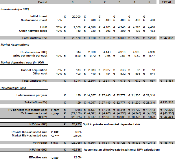
EXAMPLE 1: An initial network investment of 20 mio euro needs to be committed to provide a new service for the customer base. It is assumed that sustenance investment per year amounts to 2% of the initial investment and that operations & maintenance is 20% of the accumulated investment (50% in initial year). Other network cost, such as transmission (assumes centralized platform solution) increases with 10% per year due to increased traffic with an initial cost of €150 thousand. The total network investment and cost structure should be discounted according with the risk-free rate (assumed to be 5%). Market assumptions: s-curve consistent growth assumed with a saturation of 5 Million service users after approximately 3 years. It has been assumed that the user pays 0.8 euro per month for the service and that the service price decreases with 10% per year. Cost of acquisition assumed to be 1 euro per customer, increasing with 5% per year. Other market dependent cost assumed initially to be €400 thousand and to increase with 10% per year. It is assumed that the project is terminated after 5 years and that the terminal value amounts to 0 euro. PV stands for present value and FV for future value. The PV has been discounted back to year 0. It can be seen from the table that the project breaks-even after 3 years. The first analysis presents the NPV results (over a 5 year period) when differentiating between private (private risk-adjusted rate) and market (market risk-adjusted rate) risk taking, a positive NPV of €26M is found. This should be compared with the standard approach assuming an effective rate of 12.5%, which (not surprisingly) results in a positive NPV of €46M. The difference between the two approaches amounts to about €19M.

Example above compares the approach of using an effective discount rate r* with an analysis that differentiates between private r_rap and market risk r_ram in the NPV calculation. The example illustrates a project valuation example of introducing a new service. The introduction results in network investments and costs in order to provide and operate the service. Future cash-flows arise from growth of customer base (i.e., service users), and is offset by market related costs. All network investments and costs are assumed to be subject to private risk and should be discounted with the risk-free rate. The market-related cost and revenues are subject to market risk and the risk-adjusted rate should be used [7]. Alternatively, all investment, costs and revenues can be treated with an effective discount rate. As seen from the example, the difference between the two valuation approaches can be substantial:

NPV = €26M for differentiated market and private risk, and
NPV = €46M using an effective discount rate (e.g., difference of €20M assuming the following discount rates r_ram = 20%, r_rap =5%, r* = 12.5%). Obviously, as r_ram –> r* and r_rap –> r* , the difference in the two valuation approaches will tend to zero.

UNCERTAINTY, RISK & VALUATION

The traditional valuation methodology presented in the previous section makes no attempt to incorporate uncertainties and risk other than the effective discount-rate r* or risk-adjusted rates r_ram/rap. It is inherent in the analysis that cash-flows, as well as the future investments and cost structure, are assumed to be certain. The first level of incorporating uncertainty into the investment analysis would be to define market scenarios with an estimated (subjective) chance of occurring. A good introduction to uncertainty and risk modeling is provided in the well-written book by D. Vose [8], S.O. Sugiyama’s training notes [3] and S. Beninga’s “Financial Modeling” [7].

The Business Analyst working on the service introduction, presented in Example 1, assesses that there are 3 main NPV outcomes for the business model; NPV₁= 45, NPV₂= 20 and NPV₃= -30. The outcomes have been based on 3 different market assumptions related to customer uptake: 1. Optimistic, 2. Base and 3. Pessimistic. The NPVs are associated with the following chances of occurrence: P₁ = 25%, P₂ = 50% and P₃ = 25%.

What would the expected net-present value be given the above scenarios?

The expected NPV (ENPV) would be ENPV=P₁×NPV₁+ P₂×NPV₂+ P₃×NPV₃=25%×45+50%×20+25%×(-30) =14. Example 2 (below) illustrates the process of obtaining the expected NPV.

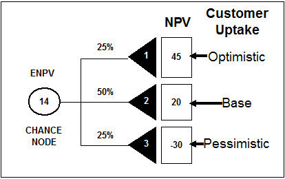
Example 2: illustrates how to calculate the expected NPV (ENPV) when 3 NPV outcomes have been identified resulting from 3 different customer uptake scenarios. The expected NPV calculation assumes that we do not have any flexibility to avoid any of the 3 outcomes. The circular node represents a chance node yielding the expected outcome given the weighted NPVs.

In general the expected NPV can be written as

$ENPV = \sum\limits_{i = 1}^N {NP{V_i} \times {P_i}}$

,where N is number of possible NPV outcomes, NPV_iis the net present value of the i^th outcome and P_i is the chance that the i^th outcome will occur. By including scenarios in the valuation analysis, the uncertainty of the real world is being captured. The risk of overestimating or underestimating a project valuation is thereby minimized. Typically, the estimation of P, which is the chance or probability, for a particular outcome is based on subjective “feeling” of the Business Analyst, who obviously still need to build a credible story around his choices of likelihood for the scenarios in questions. Clearly this is not a very satisfactory situation as all kind of heuristic biases are likely to influence the choice of a given scenarios likelihood. Still it is clearly more realistic than a purely deterministic approach with only one locked-in happening.

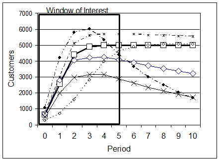
Example 3 shows various market outcomes used to study the uncertainty of market conditions upon the net-present value of Example 1and the project valuation subject these uncertainties. The curve represented by the thick solid line and open squares is the base market scenario used in Example 1, while the other curves represent variations to the base case. Various uncertainties of the customer growth have been explored. An s-curve (logistic function) approach has been used to model the customer uptake of for the studied service: $S(t) = \frac{{{S_{\max }}}}{{1 + b\,Exp( - a\,t)}}Exp[ - c\,max\left\{ {0,\left. {t - {t_d}} \right\}} \right.]$ , t is time period, S_max is the maximum expected number of customer, be determines the slope in the growth phase, and (1/a) is the years to reach the mid-point of the S-curve. The $Exp[ - c\;\max \{ 0,t - {t_d}\} ]$ function models the possible decline in customer base, with c being the rate of decline in the market share, and t_d the period when the decline sets in. S_max has been varied between 2.5 and 6.25 Million customers, with an average of 5.0 Million, b was chosen to be 50 (arbitrarily), (1/a) was varied between 1/3 and 2 (year), with a mean of 0.5 (year). In modeling the market decline, the rate of decline c was varied between 0% and 25% years, with a chosen mean value of 10%, and the t_d was varied between 0 and 3 years with a mean of 2 years before market decline starts. In all cases a so-called pert distribution was used to model the parameter variance. Instead of running a limited number of scenarios as shown in Example 2 (3 outcomes), a Monte Carlo (MC) simulation is carried out sampling several thousands of possible outcomes.

As already discussed a valuation analysis often involves many uncertain variables and assumptions. In the above Example 3 different NPV scenarios had been identified, which resulted from studying the customer uptake. Typically, the identified uncertain input variables in a simplified scenario-sensitivity approach would each have at least three possible values; minimum (x), base-line or most-likely (y), and maximum (z). For every uncertain input variable the Analyst has identified a ${\left\{ {{x_i},{y_i},{z_i}} \right\}_i}$ variation, i.e., 3 possible variations. For an analysis with 2 uncertain input variables, each with ${\left\{ {{x_i},{y_i},{z_i}} \right\}_i}$ variation, it is not difficult to show that the outcome is 9 different scenario-combinations, for 3 uncertain input variables the result is 72 scenario-combinations, 4 uncertain input variables results in 479 different scenario permutations, and so forth. In complex models containing 10 or more uncertain input variables, the number of combinations would have exceeded 30 Million permutations [9]. Clearly, if 1 or 2 uncertain input variables have been identified in a model the above presented scenario-sensitivity approach is practical. However, the range of possibilities quickly becomes very large and the simple analysis breaks down. In these situations the Business Analyst should turn to Monte Carlo [10] simulations, where a great number of outcomes and combinations can be sampled in a probabilistic manner and enables proper statistical analysis. Before the Analyst can perform an actual Monte Carlo simulation, a probability density function (pdf) needs to be assigned to each identified uncertain input variable and any correlation between model variables needs to be addressed. It should be emphasized that with the help of subject-matter experts, an experienced Analyst in most cases can identify the proper pdf to use for each uncertain input variable. A tool such as Palisade Corporation’s @RISK toolbox [2] for MS Excel visualizes, supports and greatly simplifies the process of including uncertainty into a deterministic model, and efficiently performs Monte Carlo simulations in Microsoft Excel.

Rather than guessing a given scenarios likelihood, it is preferable to transform the deterministic scenarios into one probabilistic scenario. Substituting important scalars (or drivers) with best practice probability distributions and introduce logical switches that mimic choices or options inherent in different driver outcomes. Statistical sampling across simulated outcomes will provide an effective (or blended) real option value.

In Example 1a standard deterministic valuation analysis was performed for a new service and the corresponding network investments. The inherent assumption was that all future cash-flows as well as cost-structures were known. The analysis yielded a 5-year NPV of 26 mio (using the market-private discount rates). This can be regarded as a pure deterministic outcome. The Business Analyst is requested by Management to study the impact on the project valuation incorporating uncertainties into the business model. Thus, the deterministic business model should be translated into a probabilistic model. It is quickly identified that the market assumptions, the customer intake, is an area which needs more analysis. Example 3shows various possible market outcomes. The reference market model is represented by the thick-solid line and open squares. The market outcome is linked to the business model (cash-flows, cost and net-present value). The deterministic model in Example 1 has now been transformed into a probabilistic model including market uncertainty.

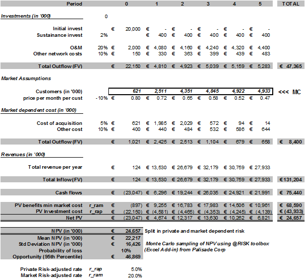
Example 4: shows the impact of uncertainty in the marketing forecast of customer growth on the Net Present Value (extending Example 1). A Monte Carlo (MC) simulation was carried out subject to the variations of the market conditions (framed box with MC in right side) described above (Example 2) and the NPV results were sampled. As can be seen in the figure above an expected mean NPV of €22M was found with a standard deviation of €16M. Further, analysis reveals a 10% probability of loss (i.e., NPV £ 0 euro) and an opportunity of up to €46M. Charts below (Example 4b and 4c) show the NPV probability density function and integral (probability), respectively.

Example 4b Example 4c

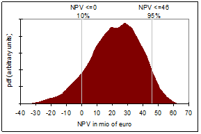
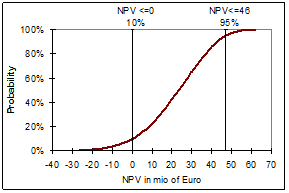
Example 4 above summarizes the result of carrying out a Monte Carlo (MC) simulation, using @RISK [2], determining the risks and opportunities of the proposed service and therefore obtaining a better foundation for decision making. In the previous examples the net-present value was represented as a single number; €26M in Example 1 and an expect NPV of €14M in Example 2. In Example 4, the NPV is far richer (see the probability charts of NPV at the bottom of the page) – first note that the mean NPV of €22M agree well with Example 1. Moreover, the Monte Carlo analysis shows the project down-side, that there is a 10% chance of ending up with a poor investment, resulting in value destruction. The opportunity or upside is a chance (i.e., 5%) of gaining more than €46M within a 5-year time-horizon. The project risk profile is represented with the NPV standard deviation, i.e. the project volatility, of €16M. It is Management’s responsibility to weight the risk, downside as well as upside, and ensure that proper mitigation will be considered to reduce the impact of the project downside and potential value destruction.

The presented valuation methodologies so far do not consider flexibility in decision making. Once an investment decision has been taken investment management is assumed to be passive. Thus, should a project turn out to destroy value, which is inevitable if revenue growth becomes limited compared to the operating cost, Management is assumed not to terminate or abandon this project. In reality active Investment Management and Management Decision Making does consider options and their economical and strategic value. In the following a detailed discussion on the valuation of options and the impact on decision making are presented. The Real options analysis (ROA) will be introduced as a natural extension of probabilistic cash flow and net present value analysis. It should be emphasized that ROA is based on some advanced mathematical, as well as statistical concepts, which will not be addressed in this work.

However, it is possible to get started on ROA with proper re-arrangement of the conventional valuation analysis, as well as incorporating uncertainty where ever appropriate. In the following the goal is to get the reader introduced to thinking about the value of options.

REAL OPTIONS & VALUATION

An investment option can be seen as a decision flexibility, which depending upon uncertain conditions, might be realized. It should be emphasized, that as with a financial option, it is at the investor’s discretion to realize an option. Any cost or investment for the option itself can be viewed as the premium a company has to pay in order to obtain the option. For example, a company could be looking at an initial technology investment, with the option later on to expand should market conditions be favorable for value growth. Exercising the option, or making the decision to expand the capacity, results in a commitment of additional cost and capital investments – the “strike price” – into realizing the plan/option. Once the option to expand has been exercised, the expected revenue stream becomes the additional value subject to private and market risks. In every technology decision a decision-maker is faced with various options and would need to consider the ever-prevalent uncertainty and risk of real-world decisions.

In the following example, a multinational company is valuing a new service with the idea to commercially launch in all its operations. The cash-flows, associated with the service, are regarded as highly uncertain, and involve significant upfront development cost and investments in infrastructure to support the service. The company studying the service is faced with several options for the initial investment as well as future development of the service. Firstly, the company needs to make the decision to launch the service in all countries in which it is based, or to start-up in one or a few countries to test the service idea before committing to a full international deployment, investing in transport and service capacity. The company also needs to evaluate the architectural options in terms of platform centralization versus de-centralization, platform supplier harmonization or commit to a more-than-one-supplier strategy. In the following, options will be discussed in relation to the service deployment as well as the platform deployment, which supports the new service. In the first instance the Marketing strategy defines a base-line scenario in which the service is launched in all its operations at the same time. The base-line architectural choice is represented by a centralized platform scenario placed in one country, providing the service and initial capacity to the whole group.

Platform centralization provides for an efficient investment and resourcing; instead of several national platform implementation projects only one country focuses its resources. However, the operating costs might be higher due to need for international leased transmission connectivity to the centralized platform. Due to the uncertainty in the assumed cash-flows, arising from market uncertainties, the following strategy has been identified; The service will be launched initially in a limited number of operations (one or two) with the option to expand should the service be successful (option 1), or should the service fail to generate revenue and growth potential an option to abandon the service after 2 years (option 2). The valuation of the identified options should be assessed in comparison with the base-line scenario of launching the service in all operations. It is clear that the expansion option (option 1) leads to a range of options in terms of platform expansion strategies depending on the traffic volume and cost of the leased international transmission (carrying the traffic) to the centralized platform.

For example, if the cost of transmission exceeds the cost of operating the service platform locally an option to locally deploy the service platform is created. From this example it can be seen that by breaking up the investment decisions into strategic options the company has ensured that it can abandon should the service fail to generate the expected revenue or cash-flows, reducing loses and destruction of wealth. However, more importantly the company, while protecting itself from the downside, has left open the option to expand at the cost of the initial investment. It is evident that as the new service has been launched and cash-flows start being generated (or lack of appropriate cash-flows) the company gains more certainty and better grounds for making decisions on which strategic options should be exercised.

In the previous example, an investment and its associated valuation could be related to the choices which come naturally out of the collection of uncertainties and the resulting risk. In the literature (e.g., [11], [12]) it has been shown that conventional cash-flow analysis, which omits option valuation, tends to under-estimate the project value [13]. The additional project value results from identifying inherent options and valuing these options separately as strategic choices that can be made in a given time-horizon relevant to the project. The consideration of the value of options in the physical world closely relates to financial options theory and treatment of financial securities [14]. The financial options analysis relates to the valuation of derivatives [15] depending on financial assets, whereas the analysis described above identifying options related to physical or real assets, such as investment in tangible projects, is defined as real options analysis (ROA). Real options analysis is a fairly new development in project valuation (see [16], [17], [18], [19], [20], and [21]), and has been adopted to gain a better understanding of the value of flexibility of choice.

One of the most important ideas about options in general and real options in particular, is that uncertainty widens the range of potential outcomes. By proper mitigation and contingency strategy the downside of uncertainty can be significantly reduced, leaving the upside potential. Uncertainty, often feared by Management, can be very valuable, provided the right level of mitigation is exercised. In our industry most committed investments involve a high degree of uncertainty, in particular concerning market forces and revenue expectations, but also technology-related uncertainty and risk is not negligible. The value of an option, or strategic choice, arises from the uncertainty and related risk that real-world projects will be facing during their life-time. The uncertain world, as well as project complexity, results in a portfolio of options, or choice-path, a company can choose from. It has been shown that such options can add significant value to a project – however, presently options are often ignored or valued incorrectly [11–21]. In projects, which are inherently uncertain, the Analyst would look for project-valuable options such as, for example:

Defer/Delay – wait and see strategy (call option)
Future growth/ Expand/Extend – resource and capacity expansion (call option)
Replacement – technology obsolescence/end-of-life issues (call option)
Introduction of new technology, service and/or product (call option)
Contraction – capacity decommissioning (put option)
Terminate/abandon – poor cash-flow contribution or market obsolescence (put option)
Switching options – dynamic/real-time decision flexibility (call/put option)
Compound options – phased and sequential investment (call/put option)

It is instructive to consider a number of examples of options/flexibilities which are representative for the mobile telecommunications industry. Real options or options on physical assets can be divided in to two basic types – calls and puts. A call option gives, the holder of the option, the right to buy an asset, and a put option provides the holder with the right to sell the underlying asset.

First, the call option will be illustrated with a few examples: One of the most important options open to management is the option to Defer or Delay (1) a project. This is a call option, right to buy, on the value of the project. The defer/delay option will be addressed at length later in this paper. The choice to Expand (2) is an option to invest in additional capacity and increase the offered output if conditions are favorable. This is defined as a call option, i.e., the right to buy or invest, on the value of the additional capacity that could enable extra customers, minutes-of-use, and of course additional revenue. The exercise price of the call option is the investment and additional cost of providing the additional capacity discounted to the time of the option exercise. A good example is the expansion of a mobile switching infrastructure to accommodate an increase in the customer base. Another example of expansion could be moving from platform centralization to de-centralization as traffic grows and the cost of centralization becomes higher than the cost of decentralizing a platform. For example, the cost of transporting traffic to a centralized platform location could, depending on cost-structure and traffic volume, become un-economical. Moreover, Management is often faced with the option to extend the life of an asset by re-investing in renewal – this choice is a so-called Replacement Option (3). This is a call option, the right to re-invest, on the assets future value. An example could be the renewal of the GSM base-transceiver stations (BTS), which would extend the life and adding additional revenue streams in the form of options to offer new services and products not possible on the older equipment. Furthermore, there might be additional value in reducing operational cost of old equipment, which typically would have higher running cost, than with new equipment. Terminate/Abandonment (5) in a project is an option to either sell or terminate a project. It is a so-called put option, i.e., it gives the holder the right to sell, on the projects value. The strike price would be the termination value of the project reduced by any closing-down costs. This option mitigates the impact of a poor investment outcome and increases the valuation of the project. A concrete example could be the option to terminate poorly revenue generating services or products, or abandon a technology where the operating costs results in value destruction. The growth in cash-flows cannot compensate the operating costs. Contraction choices (6) are options to reduce the scale of a project’s operation. This is a put option, right to “sell”, on the value of the lost capacity. The exercise price is the present value of future cost and investments saved as seen at the time of exercising the option. In reality most real investment projects can be broken up in several phases and therefore also will consist of several options and the proper investment and decision strategy will depend on the combination these options. Phased or sequential investment strategies often include Compounded Options (8), which are a series of options arising sequentially.

The radio access network site-rollout investment strategy is a good example of how compounded options analysis could be applied. The site rollout process can be broken out in (at least) 4 phases: 1. Site identification, 2. Site acquisition, 3. Site preparation (site build/civil work), and finally 4. Equipment installation, commissioning and network integration. Phase 2 depends on phase 1, phase 3 depends on phase 2, and phase 4 depends on phase 3 – a sequence of investment decisions depending on the previous decision, thus the anatomy of the real options is that of Compound Options (8) . Assuming that a given site location has been identified and acquired (call option on the site lease), which is typically the time-consuming and difficult part of the overall rollout process; the option to prepare the site emerges (Phase 3). This option, also a call option, could depend on the market expectations and the competitions strategy, local regulations and site-lease contract clauses. The flexibility arises from deferring/delaying the decision to commit investment to site preparation. The decision or option time-horizon for this deferral/delay option is typically set by the lease contract and its conditions. If the option expires the lease costs have been lost, but the value arises from not investing in a project that would result in negative cash-flow. As market conditions for the rollout technology becomes more certain, higher confidence in revenue prospects, a decision to move to site preparation (Phase 3) can be made. In terms of investment management after Phase 3 has been completed there is little reason not to pursue Phase 4 and install and integrate the equipment enabling service coverage around the site location. If at the point of Phase 3 the technology or supplier choice still remains uncertain it might be a valuable option to await (deferral/delay option) a decision on supplier and/or technology to be deployed. In the site-rollout example described other options can be identified, such as abandon/terminate option on the lease contract (i.e., a put option). After Phase 4 has been completed there might come a day where an option to replace the existing equipment with new and more efficient / economical equipment arises. It might even be interesting to consider the option value of terminating the site altogether and de-install the equipment. This could happen when operating costs exceeds the cash-flow. It should be noted that the termination option is quite dramatic with respect to site-rollout as this decision would disrupt network coverage and could aggress existing customers. However, the option to replace the older technology and maybe un-economical services with a new and more economical technology-service option might prove valuable. Most options are driven by various sources of uncertainty. In the site-rollout example, uncertainty might be found with respect to site-lease cost, time-to-secure-site, inflation (impacting the site-build cost), competition, site supply and demand, market uncertainties, and so forth

Going back to Example 1 and Example 4, the platform subject-matter expert (often different from the Analyst) has identified that if the customer base exceeds 4 Million customers and expansion of €10M will be needed. Thus, the previous examples underestimate the potential investments in platform expansion due to customer growth. Given that the base-line market scenario does identify that that this would be the case in the 2nd year of the project the €10M is included in the deterministic conventional business case for the new service. The result of including the €10M in the 2^nd year of Example 1 is that the NPV drops from €26M to €8.7M (∆NPV minus €17.6M). Obviously, the conventional Analyst would stop here and still be satisfied that this seems to be a good and solid business case. The approach of Example 4 is applied to the new situation, subject to the same market uncertainty given in Example 3. From the Monte Carlo simulation, it is found that the NPV mean-value only is €4.7M. However, the downside is that the probability of loss (i.e., an NPV less than 0) now is 38%. It is important to realize that in both examples is the assumption that there is no choice or flexibility concerning the €10M investment; the investment will be committed in year two. However, the project has an option – the option to expand provided that the customer base exceeds 4 Million customers. Time wise it is a flexible option in the sense that if the project expected lifetime is 5 years, any time within this time-horizon is there a possibility that the customer base exceeds the critical mass for platform expansion.

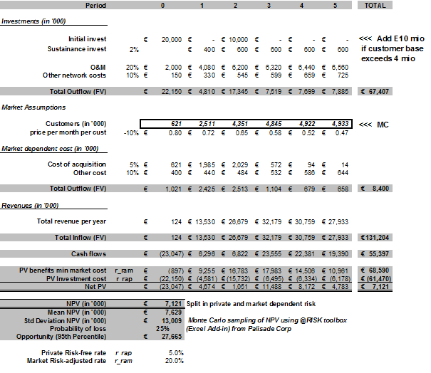
Example 5: Shows the NPV valuation outcome when an option to expand is included in the model of Example 4. The €10M is added if and only if the customer base exceeds 4 Million.

In the above Example 5 the probabilistic model has been changed to add €10M if and only if the customer base exceeds 4 Million. Basically, the option of expansion is being simulated. Treating the expansion as an option is clearly valuable for the business case, as the NPV mean-value has increased from €4.7M to €7.6M. In principle the option value could be taken to €2.9M. It is worthwhile noticing that the probability of loss (from 38% to 25%) has also been reduced by allowing for the option not to expand the platform if the customer base target is not achieved. It should be noted that although the example does illustrate the idea of options and flexibility it is not completely in line with a proper real options analysis.

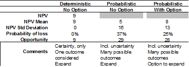
Example 6 Shows the different valuation outcomes depending on whether the €10M platform expansion (when customer base exceeds 4 Million) is considered as un-avoidable (i.e., the “Deterministic No Option” and “Probabilistic No Option”) or as an option or choice to do so (“Probabilistic with Option”). It should be noted that the additional €3M in difference between “Probabilistic No Option” and “Probabilistic With Option” can be regarded as an effective option value, but it does not necessarily agree with a proper real-option valuation analysis of the option to expand. Another difference in the two probabilistic models is that in the model with option to expand an expansion can happen any year if customer base exceeds 4 Million, while the No option model only considers the expansion in year 2 where according with the marketing forecast the base exceeds the 4 Million. Note that Example 6 is different in assumptions than Example 1 and Example 4 as these do not include the additional €10M.

Example 6 above summarizes the three different approaches of valuation analysis; deterministic (essential 1-dimensional), probabilistic with options, and probabilistic including value options.

The investment analysis of real options as presented in this paper is not a revolution but rather an evolution of the conventional cash-flow and NPV analysis. The approach to valuation is first to understand and proper model the base-line case. After the conventional analysis has been carried out, the analyst, together with subject-matter experts, should determine areas of uncertainty by identifying the most relevant uncertain input parameters and their variation-ranges. As described in the previous section the deterministic business model is being transformed into a probabilistic model. The valuation range, or NPV probability distribution, is obtained by Monte Carlo simulations and the opportunity and risk profile is analyzed. The NPV opportunity-risk profile will identify the need for mitigation strategies, which in itself result in studying the various options inherent in the project. The next step in the valuation analysis is to value the identified project or real options. The qualitatively importance of considering real options in investment decisions has been provided in this paper. It has been shown that conventional investment analysis, represented by net-present value and discounted cash-flow analysis, gives only one side of the valuation analysis. As uncertainty is the “farther” of opportunity and risk it needs to be considered in the valuation process. Are identified options always valuable? The answer to that question is no – if we have certainty about an option movement is not in our favor then the option would be valuable. Think for example of considering a growth option at the onset of severe recession.

The real options analysis is often presented as being difficult and too mathematical; in particular

due to the involvement of the partial differential equations (PDE) that describes the underlying uncertainty (continuous-time stochastic processes, involvement of Markov processes, diffusion processes, and so forth). Studying PDEs are the basis for the ground-breaking work of the Black-Scholes-Merton [22] [23] on option pricing, which provided the financial community with an analytical expression for valuing financial options. However, “heavy” mathematical analysis is not really needed for getting started on real option.

Real options are a way of thinking, identifying valuable options in a project or potential investment that could create even more value by considering as an option instead of a deterministic given.

Furthermore, Cox et al [24] proposed a simplified algebraic approach, which involves so-called binominal trees representing price, cash-flow, or value movements in time. The binomial approach is very easy to understand and implement, resembling standard decision tree analysis, and visually easy to generate, as well as algebraically straightforward to solve.

SUMMARY

Real options are everywhere where uncertainty governs investment decisions. It should be clear that uncertainty can be turned into a great advantage for value growth providing proper contingencies are taken for reducing the downside of uncertainty – mitigating risk. Very few investment decisions are static, as conventional discounted cash-flow analysis otherwise might indicate, but are ever changing due to changes in market conditions (global as well as local), technologies, cultural trends, etc. In order to continue to create wealth and value for the company value growth is needed and should force a dynamic investment management process that continuously looks at the existing as well as future valuable options available for the industry. It is compelling to say that a company’s value should be related to its real-options portfolio, and its track record in mitigating risk, and achieving the uncertain up-side of opportunities.

ACKNOWEDGEMENT

I am indebted to Sam Sugiyama (President & Founder of EC Risk USA & Europe) for taking time out from a very busy schedule and having a detailed look at the content of our paper. His insights and hard questions have greatly enriched this work. Moreover, I would also like to thank Maurice Ketel (Manager Network Economics), Jim Burke (who in 2006 was Head of T-Mobile Technology Office) and Norbert Matthes (who in 2007 was Head of Network Economics T-Mobile Deutschland) for their interest and very valuable comments and suggestions.

___________________________

APPENDIX – MATHEMATICS OF VALUE.

Firstly we note that the Future Value FV (of money) can be defined as the present Value PV (of money) times a relative increase given by an effective rate r* (i.e., that represents the change of money value between time periods), reflecting value increase or of course decrease over a cause of time t;

$F{V_t} = {(1 + r*)^t}\;PV$

So the Present Value given we know the Future Value would be

$PV = \frac{{F{V_t}}}{{{{(1 + r*)}^t}}}$

For a sequence (or series) of future money flow we can write the present value as

$PV = \sum\limits_{t = 1}^N {\frac{{F{V_t}}}{{{{(1 + r*)}^t}}}}$

If r* is positive time-value-of-money follows naturally, i.e., money received in the future is worth less than today. It is a fundamental assumption that you can create more value with your money today than waiting to get them in the future (i.e., not per se right for majority of human beings but maybe for Homo Economicus).

First the sequence of future money value (discounted to the present) has the structure of a geometric series: ${V_n} = \sum\limits_{k = 0}^n {\frac{{{y_k}}}{{{{\left( {1 + r} \right)}^k}}}}$ , with y_k+1 = g*y_k (i.e., g* representing the change in y between two periods k and k+1).

Define ${a_k} = \frac{{{y_k}}}{{{{\left( {1 + r} \right)}^k}}}$ and note that $\frac{{{a_{k + 1}}}}{{{a_k}}} = \frac{{g*}}{{1 + r}} = \frac{{1 + g}}{{1 + r}} = s$ , thus in this framework we have that ${V_n} = \sum\limits_{k = 0}^n {{s^k}}$ (note: I am doing all kind of “naughty” simplifications to not get too much trouble with the math).

The following relation is easy to realize:

$\begin{array}{l} {V_n} = 1 + s + {s^2} + {s^3} + .......... + {s^n}\\ s{V_n} = s + {s^2} + {s^3} + .......... + {s^n} + {s^{n + 1}} \end{array}$ , subtract the two equations from each other and the result is $(1 - s){V_n} = (1 - {s^{n + 1}})\quad \Leftrightarrow \quad {V_n} = \frac{{1 - {s^{n + 1}}}}{{1 - s}}\quad \Leftrightarrow$ $\quad {V_n} = \frac{{1 + r}}{{r - g}} - \frac{{(1 + g)}}{{r - g}}{\left( {\frac{{1 + g}}{{1 + r}}} \right)^n}$

. In the limit where n goes toward infinity (¥), providing that $\left| s \right| < 1\quad \Leftrightarrow \quad \left| {\frac{{1 + g}}{{1 + r}}} \right| < 1$ , it can be seen that .

It is often forgotten that this only is correct if and only if $\left| {1 + g} \right| < \left| {1 + r} \right|$ or in other words, if the discount rate (to present value) is higher than the future value growth rate. ${V_\infty } = \frac{1}{{1 - s}}\quad \Leftrightarrow \quad {V_\infty } = \frac{{1 + r}}{{r - g}}$

You might often hear you finance folks (or M&A jockeys) talk about Terminal Value (they might also call it continuation value or horizon value … for many years I called it Termination Value … though that’s of course slightly out of synch with Homo Financius not to be mistaken for Homo Economicus :-).

$PV = \sum\limits_{t = 1}^T {\frac{{FV{}_t}}{{{{(1 + r*)}^t}}}} + T{V_{T \to \infty }} = NP{V_T} + \sum\limits_{t = T + 1}^\infty {\frac{{FV{}_t}}{{{{(1 + r*)}^t}}}}$ with TV representing the Terminal Value and

NPV representing the net present value as calculated over a well-defined time span T.

I always found the Terminal Value fascinating as the size (matters?) or relative magnitude can be very substantial and frequently far greater than the NPV in terms of “value contribution” to the present value. Of course we do assume that our business model will survive to “Kingdom Come”. Appears to be a slightly optimistic assumptions (n’est pas mes amis? :-). We also assume that everything in the future is defined by the last year of cash-flow, the cash flow growth rate and our discount rate (hmmm don’t say that Homo Financius isn’t optimistic). Mathematically this is all okay (if $\left| {1 + g} \right| < \left| {1 + r} \right|$ ), economically maybe not so. I have had many and intense debates with past finance colleagues about the validity of Terminal Value. However, to date it remains a fairly standard practice to joggle up the enterprise value of a business model with a “bit” of Terminal Value.

Using the above (i.e., including our somewhat “naughty” simplifications)

$TV = \sum\limits_{t = T + 1}^\infty {\frac{{{y_t}}}{{{{(1 + r)}^t}}}}$

$TV = \frac{{(1 + g)\,{y_T}}}{{{{(1 + r)}^{T + 1}}}}\sum\limits_{j = 0}^\infty {\frac{{{{(1 + g)}^j}}}{{{{(1 + r)}^j}}}}$

$TV \approx \frac{{(1 + g)\,{y_T}}}{{(r - g)\,{{(1 + r)}^T}}}\quad \forall \,\left| {1 + g} \right| < \left| {1 + r} \right|$

It is easy to see why TV can be a very substantial contribution to the total value of a business model. The denominator (r-g) tends to be a lot smaller than 1 (i.e., note that always we have g<r) and though “blows” up the TV contribution to the present value (even when g is chosen to be zero).

Let’s evaluate the impact on uncertainty of the interest rate x, first re-write the NPV formula:

$NP{V_n} = {V_n} = \sum\limits_{k = 0}^n {\frac{{{y_k}}}{{{{\left( {1 + x} \right)}^k}}}}$ , y_k is the cash-flow of time k (for the moment it remains unspecified), from

error/uncertainty propagation it is known that the standard deviation can be written as $\Delta {z^2} = {\left( {\frac{{\partial f}}{{\partial x}}} \right)^2}\Delta {x^2} + {\left( {\frac{{\partial f}}{{\partial y}}} \right)^2}\Delta {y^2} + ....$ , where z=f(x,y,z,…) is a multi-variate function. Identifying the terms in the NPV formula is easy: z = V_n and $f(x,\left\{ {{y_k}} \right\};k) = \sum\limits_k {\frac{{{y_k}}}{{{{\left( {1 + x} \right)}^k}}}}$

In the first approximation assume that x is the uncertain parameter, while y_k is certain (i.e., ∆y_k=0), then the following holds for the NPV standard deviation:

${\left( {\Delta {V_n}} \right)^2} = {\left( {\sum\limits_{k = 0}^n {\frac{{k{y_k}}}{{{{\left( {1 + x} \right)}^{k + 1}}}}} } \right)^2}{\left( {\Delta x} \right)^2}\quad \Leftrightarrow$ $\Delta {V_n} = \left| {\Delta x} \right|\left| {\sum\limits_{k = 0}^n {\frac{{k{y_k}}}{{{{(1 + x)}^{k + 1}}}}} } \right|$ ,

in the special case where y_k is constant for all k’s,. It can be shown (similar analysis as above) that

$\Delta {V_n} = \left| {\Delta x} \right|\left| {{y_n}} \right|\left| {\frac{{1 - {r^{n + 1}}}}{{{{(1 - r)}^2}}} - \frac{{1 + n\,{r^{n + 1}}}}{{(1 - r)}}} \right|$ with $r = \frac{1}{{1 + x}}$ .

In the limit where n goes toward infinity, applying l’Hospital’s rule showing that $n\,{r^{n + 1}} \to 0\;for\;n \to \infty$ , the following holds for propagating uncertainty/errors in the NPV formula:

$\Delta {V_\infty } = \left| {\Delta x} \right|\,\left| y \right|\;\left| {\frac{1}{{{{\left( {1 - r} \right)}^2}}} - \frac{1}{{(1 - r)}}} \right|$ $= \left| {\Delta x} \right|\,\left| y \right|\;\left| {\frac{{ - r}}{{{{(1 - r)}^2}}}} \right| = \left| {\Delta x} \right|\,\left| y \right|\;\left| {\frac{{1 + x}}{{{x^2}}}} \right|$

Let’s take a numerical example, y=1, the interest rate x = 10% and the uncertainty/error is assumed to be no more than ∆x=3% (7%£ x £13%), assume that n®¥ (infinite time-horizon). Using the formula derived above NPV_¥=11 and ∆NPV_¥=±3.30 or a 30% error on estimated NPV. If the assumed cash-flows (i.e., y_k) also uncertain the error will even be greater than 30%. The above analysis becomes more complex when y_k is non-constant over time k and as y_k to should be regarded as uncertain. The use of for example Microsoft Excel becomes rather useful to gain further insight (although the math is pretty fun too).

[1] This is likely due to the widespread use of MS Excel and financial pocket calculators allowing for easy NPV calculations, without the necessity for the user to understand the underlying mathematics, treating the formula as “black” box calculation. Note a common mistake using MS Excel NPV function is to include initial investment (t=0) in the formula – this is wrong the NPV formula starts with t=1. Thus, initial investment would be discounted which would lead to an overestimation of value.

[2] http://www.palisade-europe.com/. For purchases contact Palisade Sales & Training, The Blue House 30, Calvin Street, London E1 6NW, United Kingdom, Tel. +442074269955, Fax +442073751229.

[3] Sugiyama, S.O., “Risk Assessment Training using The Decision Tools Suite 4.5 – A step-by-step Approach” and “Introduction to Advanced Applications for Decision Tools Suite – Training Notebook – A step-by-step Approach”, Palisade Corporation. The Training Course as well as the training material itself can be highly recommended.

[4] Most people in general not schooled in probability theory, statistics and mathematical analysis. Great care should be taken to present matters in an intuitive rather than mathematical fashion.

[5] Hill, A., “Corporate Finance”, Financial Times Pitman Publishing, London, 1998.

[6]This result comes straight from geometric series calculus. Remember a geometric series is defined as, where is constant. For the NPV geometric series it can easily be shown that, r being the interest rate. A very important property is that the series converge if, which is the case for the NPV formula when the interest rate r>1. The convergent series sums to a finite value of for k starting at 1 and summed up to ¥ (infinite).

[7] Benninga, S., “Financial Modeling”, The MIT Press, Cambridge Massachusetts (2000), pp.27 – 52. Chapter 2 describes procedures for calculating cost of capital. This book is the true practitioners guide to financial modeling in MS Excel.

[8] Vose, D., “Risk Analysis A Quantitative Guide”, (2^nd edition), Wiley, New York, 2000. A very competent book on risk modeling with a lot of examples and insight into competent/correct use of probability distribution functions.

[9] The number of scenario combinations are calculated as follows: an uncertain input variable can be characterized by the following possibility setwith length s, in case of k uncertain input variables the number of combinations can be calculated as , where is the COMBIN function of Microsoft Excel.

[10] A Monte Carlo simulation refers to the traditional method of sampling random (stochastic) variables in modeling. Samples are chosen completely randomly across the range of the distribution. For highly skewed or long-tailed distributions a large numbers of samples are needed for convergence. The @Risk product from Palisade Corporation (see http://www.palisade.com) supplies the perfect tool-box (Excel add-in) for converting a deterministic business model (or any other model) into a probabilistic one.

[11] Luehrman, T.A., “Investment Opportunities as Real Options: Getting Started with the Numbers”, Harvard Business Review, (July – August 1998), p.p. 3-15.

[12] Luehrman, T.A., “Strategy as a Portfolio of Real Options”, Harvard Business Review, (September-October 1998), p.p. 89-99.

[13] Providing that the business assumptions where not inflated to make the case positive in the first place.

[14] Hull, J.C., “Options, Futures, and Other Derivatives”, 5^th Edition, Prentice Hall, New Jersey, 2003. This is a wonderful book, which provides the basic and advanced material for understanding options.

[15] A derivative is a financial instrument whose price depends on, or is derived from, the price of another asset.

[16] Boer, F.P., “The Valuation of Technology Business and Financial Issues in R&D”, Wiley, New York, 1999.

[17] Amram, M., and Kulatilaka, N., “Real Options Managing Strategic Investment in an Uncertain World”, Harvard Business School Press, Boston, 1999. Non-mathematical, provides a lot of good insight into real options and qualitative analysis.

[18] Copeland, T., and V. Antikarov, “Real Options: A Practitioners Guide”, Texere, New York, 2001. While the book provides a lot of insight into the area of practical implementation of Real Options, great care should be taken with the examples in this book. Most of the examples are full of numerical mistakes. Working out the examples and correcting the mistakes provides a great mean of obtaining practical experience.

[19] Munn, J.C., “Real Options Analysis”, Wiley, New York, 2002.

[20] Amram. M., “Value Sweep Mapping Corporate Growth Opportunities”, Harvard Business School Press, Boston, 2002.

[21] Boer, F.P., “The Real Options Solution Finding Total Value in a High-Risk World”, Wiley, New York, 2002.

[22]] Black, F., and Scholes, M., “The Pricing of Options and Corporate Liabilities”, Journal of Political Economy, 81 (May/June 1973), pp. 637-659.

[23] Merton, J.C., “Theory of Rational Option Pricing”, Bell Journal of Economics and Management Science, 4 (Spring 1973), 141-183.

[24] Cox, J.C., Ross, S.A., and Rubinstein, M., “Option Pricing: A Simplified Approach”, Journal of Financial Economics, 7 (October 1979) pp. 229-63.

GSM – Gone So Much … or is it?

Posted on January 18, 2014 by Dr. Kim

A Billion GSM subscriptions & almost $200 Billion GSM revenue will have gone within the next 5 years.
GSM earns a lot less than its “fair” share of the top-line, a trend that will further worsened going forward.
GSM revenue are fading out rapidly across a majority of the mobile markets across the Globe.
Accelerated GSM phase-out happens when pricing level of the next technology option relative to the GDP per capita drops below 2%.
220 MHz of great spectrum is tied up in GSM, just waiting to be liberated.
GSM is horrific spectral in-efficient in comparison to today’s cellular standards.
Eventually we will have 1 GSM network across a given market, shared by all operators, supporting fringe legacy devices (e.g., M2M) while allowing operators to re-purpose remaining legacy GSM spectrum.
The single Shared-GSM network might survive past any economical justification for its existence merely serving legal and political interests.

Gone So Much … GSM is ancient, uncool and so 90s … why would anybody bother with that stuff any longer … its synonymous with the Nokia Handset (which btw is also ancient, uncool and so 90s … and almost no longer among us thanks to our friend Elop …). In many emerging markets GSM-only phones are hardly demanded or sold any longer in the grey markets. Grey market that make up 90% (or more) of handset sales in many of those emerging markets. Moreover, its not only AT&T in the US talking about 2G phase-out but also an emerging market such as Thailand is believed to be void of GSM within the next couple of years.

A bit of Personal History. Some years ago I had the privilege to work with some very smart people in the Telecom Industry on merging two very big mobile operations (ca.140 million in combined customer base). One of our cardinal spectrum strategic and technology arguments were the gain in spectral efficiency such a merger would bring. Anecdotally it is worth mentioning that the technology synergies and spectrum strategic ideas largely would have financed the deal in shear synergies.

In discussions with the country’s regulator we were asked why we could not “just” switch off GSM? Then use that freed GSM spectrum for new cellular technologies, such as UMTS and even LTE. Thereby gaining sufficient spectral efficiency that merging the two business would become un-necessary. The proposal would have effectively turned off the button of a service that served at ca. 70 Million GSM-only (incl, EDGE & GPRS) subscribers (at the time) across the country. Now that would have been expensive and most likely caused a couple or thousands of class action suits to the beat.

Here is how one could have thought about the process of clearing out GSM for something better (though overall its is more for richer and poorer). There is no “just …press the off button”, as also Sprint experienced with their iDEN migration.

Our thoughts (and submitted Declarations) were that by merging the two operators spectrum (and sites pool) we could create sufficient spectral capacity to support both GSM (which we all granted was phasing out) and provide more capacity and customer experience for the Now Generation Technology (i.e., HSPA+ or 4G as they like to call it in that particular market … Heretics! ;-). A recent must read GigaOM blog by Keith Fitchard “AT&T begins cannibalizing 2G and 3G networks to boost LTE capacity” describes very well the aggressive no-nonsense thinking of US carriers (or simply desperation or both) when it comes to the quest for spectrum efficiency and enhanced customer experience (which co-incidentally also yields the best ARPUs).

It is worth mentioning that more than 2×110 Mega Hertz is tied up in GSM, Up-to 2×35 MHz at 900MHz (if E-GSM has been evoked) and 2×75 MHz at 1800MHz (yes! I am ignoring US GSM band plans, they are messed up but pretty fun nevertheless … different story for another time). Being able to re-purpose this amount of spectrum to more spectral efficient cellular technologies (e.g., UMTS Voice, HSPA+ and LTE) would clearly leapfrog mobile broadband, increase voice capacity at increased quality, and serve the current billions of GSM-only users as well as the next billion un-connected or under-server customer segments with The Internet. The macro-economical benefits being very substantial.

220 MHz of great spectrum is tied up in GSM, just waiting to be liberated.

Back in the days of 2003 I did my first detailed GSM phase-out techno-economical analysis (a bit premature one might add). I was very interested in questions such as “when can we switched off GSM?”, “what are the economical premises of exiting GSM?”, “Why do operators today still continue to encourage subscriber growth on their GSM networks?”, “Today … if you got your hands on GSM usable spectrum, would you start a GSM operation?”, “Why?” and “Why not?”, etc..

So why don’t we “just” switch off GSM? and let go of that old in-efficient cellular technology?

How in-efficient? you may ask? … Pending a little bit on what state the GSM is in, we can have ca. 3 times more voice users in WCDMA (i.e., UMTS) compared to GSM with Adaptive Multi-Rate (AMR) codec support. Newer technology releases supports even more dramatic leaps in voice handling capabilities.

Data? what about cellular data? That GSM, including its data handling enhancements GPRS and EDGE, is light-bits away from the data handling capabilities of WCDMA, HSPA+, LTE and so forth is at this point a well establish fact.

Clearly GSM is horrific spectral in-efficient in comparison to later cellular standards such as WCDMA, HSPA(+) and LTE(+) and its only light (in a very dark tunnel) is that it is supported at lower frequencies (i.e., more economical deployment in rural areas and for large surface area countries). Though today that no longer unique as UMTS and LTE are available in similar or even lower frequency ranges. … of course there are other economical issues at plays as well, which we will see below.

Why do we still bother with a 27+ year old technology? a technology that has very poor spectral efficiency in comparison with later cellular technologies. GSM after all “only” provides Voice, SMS and pretty low bandwidth mobile data (while better than nothing, still very close to nothing).

Well for one thing! there is of course the money thing? (and we know that that makes the world go around) ca. 4+ Billion GSM subscriptions worldwide (incl. GPRS & EDGE) generating a total GSM turnover of 280+ Billion US$.

In 2017 we anticipate to have a little less than 3 Billion GSM subscriptions generating ca. 100+ Billion US$. So ….a Billion GSM subscriptions and almost 200 Billion US$ GSM revenue will have dis-appeared within the next 5 years (and for the sake of mobile operators hopefully replaced by something better).

In this trend APAC, takes its lion share of the GSM subscription loss with ca. 65% (ca, 800 Million) of the total loss and ca. 50% of the GSM top-line loss (ca. 100 Billion US$).

The share of GSM revenue is rapidly declining across (almost) all markets;

The GSM revenue as share of the total revenue (as well as in absolute terms) rapidly diminishes, as 3G and LTE are introduced and customer migrate to those more modern technologies.

If the should be any doubts GSM does not get its fair share revenue compared to its share of the subscriptions (or subscribers for that matter):

While the above data does contain two main clusters, it still pretty well illustrates (what should be no real surprise to any one) that GSM earns back a lot less than its “fair” share (whatever that really means). And again if anyone would be in doubt that picture will be grimmer as the we fast forward to the near future;

Grim, Grimmer, Grimmest!

Today GSM earns a lot less than its “fair” share of the top-line, this trend will be further worsened going forward.

So we can soon phase-out GSM? Right? hmmmm! Maybe not so fast!

Well while GSM revenue has certainly declined and expected to continue the decline, in many markets the GSM-only (e.g., here defined as a customers that only have GSM Voice, GPRS and/or EDGE available) customers have not declined in proportion to the related revenue might fool us to believe.

The above statistics illustrates the GSM-only subscription share of the total cellular business.

There is more to GSM than market and revenue share … and we do need to have a look at the actual decline of GSM subscriptions (or unique users which is not per se the same) and revenue;

The GSM revenue are expected to massively free fall over the next 5 years!

However, also observe (in the chart above) that we need to sustain the network and its associated cost as a considerable amount of customers remain on the network, despite generating a lot less top line.

As we have already seen above, in the next 5 years there will be many markets where GSM subscription and subscriber share will remain reasonable strong albeit the technology’s ability to turn-over revenue will be in free-fall in most markets.

Analyzing data from Pyramid Research (actual & projection for the period 2013 to 2017), including other analyst data sets (particular on actual data), extrapolating the data beyond 2017 by diffusion models approximating the dynamics of technology migration in the various market, we can get an idea about the remaining (residual) life of GSM. In other words we can make GSM phase-out projections as well as get a feel for the terminal revenue (or residual value) left in GSM. Further get an appreciation of how that terminal value compares to the total mobile turnover over the same GSM phase-out period.

The chart below provide the results of such a comprehensive analysis. The colored bars illustrate the various years of onset of GSM phase-out; (a) the earliest year which is equal to the lower end of light-blue bar is typically the year where migration off GSM accelerates, (b) the upper end of the light-blue bar is a most-likely year where after GSM no longer would be profitable, and (c) the upper end of the red bar illustrates the maximum expected life of GSM. It should be noted that the GSM Phase-out chart below might not be shown in its entirety (particular right side of the chart). Clicking on the Chart itself will display it in full.

Taking the above GSM phase-out years, we can get a feeling for how many useful years GSM has left in terms of economical-life and customer life-time defined as which event comes first of (i) less than 1 Million GSM subscriptions or (ii) 5% GSM market-share. 2014 has been taken as the reference year;

It should be noted that the Useful Life-span of GSM chart above might not be shown in its entirety (particular right side of the chart). Clicking on the Chart itself will display it in full.

AREAS	#MARKETS	GSM – REMAINING LIFE
Western Europe	16	4.1 +/- 3.3 years
Asia Pacific	13	6.4 +/- 5.0 years
Middle East & Africa	17	11.0 +/- 6.2 years
Central Eastern Europe	8	6.9 +/- 4.8 years
Latin America	19	6.6 +/- 3.7 years

That Western Europe (and US which has not been shown here) has the most aggressive time-lines for GSM phase-out should come as no surprise. The 3G/UMTS has been deployed there the longest and the 3G price level to GDP has come down to a level where there is hardly any barrier for most mobile users to switch from GSM to UMTS. Also the WEU region has the most extensive UMTS coverage which also removes the GSM to UMTS switching barrier. Central Eastern Europe average is pulled up (i.e., longer useful life) substantial by Russia and Ukraine that shows fairly extreme laggardness in GSM phase-out (in comparison with the other CEE markets). For Middle East and Africa it should be noted that there are two very strong clusters of data distinguishing the Gulf States from the African Countries. Most of the Gulf States have only a very few years of remaining useful life of GSM. In general the GSM remaining life trend can be described fairly well with the amount of time UMTS has been in a given market (i.e., though smartphone introduction did kick-start the migration from GSM more than anything else), the extend of UMTS coverage (i.e., degree of pop and geo coverage) and the basic economics of UMTS.

In my analysis I have assumed 4 major triggers for GSM phase-out;

Analysis shows that once the 3G (or non-2G) ARPU is below 2% of the nominal GDP per capita an acceleration of migration away from GSM speeds up. I have (somewhat arbitrarily) chosen 1% as my limit where there is no longer any essential barrier of customer migrating off GSM.
When GSM penetration is below 5% as a decision point for converting (by possible subsidies) GSM customers to a more modern and efficient technology. This obviously does depend on total customer base and the local economical framework and as such is only a heuristics rather than a universal rule.
Last but not least, my 3rd criteria for phasing out GSM is when its base is below 1 million subscriptions (i.e., typically 500 to 800 thousand subscribers).
Last but not least, before complete phase-out of GSM can commence, operators obviously need to provide the alternative technology (e.g., UMTS or LTE) coverage that can replace the existing GSM coverage. This is in general only economical if comparable frequency range can be used and thus for example for UMTS coverage replacement of GSM in many cases re-farming/re-purposing 900MHz from GSM to UMTS. This last point can be a very substantial bottleneck and show stopper for migration from GSM to UMTS, particular in rural areas or in countries with very substantial rural populations on GSM.

Interestingly enough, extensive data analysis on more than 70 markets, shows that the GSM phase—out dynamics appears to have little or no dependency on (a) the 2G ARPU level, (b) 2G ARPU level relative to 3G ARPU and (c) handset pricing (although I should point out that I have not had a lot of data here to be firm in this conclusion, in particular reliable data for grey market handset pricing across the emerging markets is a challenge).

One of the important trigger points for onset of accelerated GSM phase-out is the pricing level of the next technology (e.g., 3G) option relative to the GDP per capita.

Migration decision appears less to do with the legacy price of the old technology or old technology price relative to new technology pricing.

Above chart illustrates an analysis made on 2012 actual data for more than 70+ markets all across WEU, CEE, APAC, EMEA and LA (i.e., coinciding with markets covered by Pyramid Research). It is very interesting to observe the dynamics as the markets develop into the future and the data moves towards the left indicating more affordable 3G pricing (relative to GDP per capita) and increasingly faster GSM phase-out as is evident from the chart below providing the same markets as above but fast forwarded 5 years (i.e., 2017).

Firstly the GSM ARPU level across most markets is below 2% of a given markets GDP per capita. There is no clear evidence in the country data available that the GSM ARPU development has had any effect on slowing down or accelerating GSM phase-out. Most likely an indication that GSM has reached (or will reach shortly) a cost level where customers become insensitive.

Conceptually we can visualize the GSM phase-out dynamics in the following way were as the 3G gets increasingly affordable (which may or should include the device cost depending on taste), GSM phase-out accelerates (i.e., moving from right to left in the illustrative chart below). While the chart illustration below is more attuned to emerging market migration dynamics of GSM phase-out it can of course with minor adaptations be used for other more balanced prepaid-postpaid markets.

We should keep in mind that unless the mobile operators new technology coverage (e.g., UMTS, LTE, ..) at the very least overlap the GSM coverage, the migration from GSM to UMTS (or LTE) will eventually stop. This can in countries with a substantial rural population in particular become a blocking stone for an effective 100% migration. Resulting in large areas and population share that will remain underserved (i.e., only GSM available) and thus depend on an in-efficient and ancient technology without the macro-economical benefits (i.e., boost of rural GDP) new and far more efficient cellular technologies could bring.

That’s all fine … what a surprise that customers wants better when it gets affordable (like to have wanted that even more when it was not affordable)… and that affordability is relative is hardly a surprising either.

In order for an operator to make an informed opinion about when to switch off GSM, it would need to evaluated the remaining business opportunity, or residual GSM value, against the value for re-purposing the GSM spectrum to a better technology, i.e., with a superior customer experience potential, and with a substantial higher ARPU utilization.

Counting from 2014, the remaining life-time aka terminal aka residual GSM revenue will be in the order of 850 Billion US$ … agreeable an apparently dramatic number … however, the residual GSM revenue is on average no more than 5% of total cellular turnover and for many countries a lower than that. Actual 45 markets out of the 73 studied will have a terminal GSM revenue lower than 5%.

The chart below provides an overview of the Residual GSM Revenues in Billion of US$ (on a logarithmic scale) and the percentage of Residual GSM value out of the total cellular turnover (linear scale) for 75 top markets spread across Western Europe, Central Eastern Europe, Asia Pacific, Middle East & Africa, and Latin America.

Do note that the GSM Terminal Revenue chart above might not be shown in its entirety (right side of the chart). Clicking on the Chart itself will display it in full.

It is quiet clear from the above chart that, apart from a few outliers, GSM revenue are fading out rapidly across a majority of the mobile markets across the globe. Even if the residual GSM topline might appear tempting, it obviously need to be compared to the operating expenses for sustaining the legacy technology as well as considering that a more modern technology would create higher efficiency (and possible ARPU arbitrage) and therefor mitigate margin decline sustaining more traffic and customers.

Emerging APAC MNO Example: an emerging market in APAC has 100 Million subscriptions and ca. 70 Million unique cellular user base.One of the Mobile Network Operators (MNO) in this market has approx. 33% market share (revenue share slightly larger). in 2012 its EBITDA margin was 42%. Technology cost share of overall Opex is 25% and for the sake of simplicity the corresponding GSM cost share is in 2012 assumed to be 50% of the Total Technology Opex. As the business evolves it is assumed that the GSM cost base grows slower than non-GSM technology cost elements. This particular market has a residual GSM revenue potential of approx. 4 Billion US$ and the MNO under the loop has 1.3 Billion US$ remaining GSM revenue potential.

Our analysis shows that the GSM business would start to breakdown (within the assumed economical framework or template) at around 5 Million GSM subscriptions or 3.5 Million unique users. This would happen around 2019 (+/- 2 years, with a bias towards earlier years) and thus leave the business with another 3 to 5 years of likely profitable GSM operation. See the chart below.

This illustration shows (not surprisingly) that there is a point where even if the phasing-out GSM turns-over revenue, from an economical perspective it makes no sense for a single mobile operator to keep its GSM network alive for a diminishing customer base and even faster evaporating top-line.

In the example above it is clear that the MNO should start planning for the inevitable – the demise of GSM. Having a clear GSM phase-out strategy as soon as possible and targeting GSM termination no later than 2018 to 2019 just makes pretty good sense. Looking at risks to the dynamics of the market development in this particular market there is a higher likelihood of no-profit being reached earlier rather than later.

Would it make sense to startup a new GSM business in the market above? Given the 3 to 5 years that the existing mobile operators have to meet retire GSM before it becomes un-profitable, it hardly make much sense for a Greenfield operator to get started on the GSM idea (seem to be better ways for spending cash).

However, if that Greenfield operator could become The GSM Operator for all existing MNO players in the market, allowing those legacy MNOs to re-purpose their existing GSM spectrum (and possible with a retro-active wholesale deal), then maybe in the short term it might make a little sense. However, it quiet frankly would be like peeing in your trousers on a cold winter day, it will be warm for a short while but then it really gets cold (as my Grandmother used to say).

What GSM strategies makes really sense in its autumn days?

Quit clearly GSM Network Sharing would make a lot of sense economically and operationally as it would allow re-purposing of legacy spectrum to more modern and substantially more efficient cellular technologies.

The single Shared-GSM network would act as a bridge for legacy GSM M2M devices, extreme laggards and problematic coverage areas that might not be economical to replace in the shorter – medium term. Thus mobile operators could then solve possible long-term contractual obligations to businesses and consumers having fringe devices connecting with GSM (i.e., metering, alarms, etc..). The single Shared-GSM network might very well survive for a considerable time past any economical justification for its existence merely serving legal and political interests. Thanks to Stein Erik Paulsen who pointed this problem out for GSM phase-out.

I am not (too) hanged up about the general Capex & Opex benefits of Network Sharing in this context (yet another story for another day). The compelling logical step of having 1 (ONE) GSM network across a given market, shared by all operators, supporting the phase-out of GSM while allowing to re-purpose legacy GSM spectrum for UMTS/HSPA and eventually LTE(+), is almost screamingly obvious. This furthermore would feed a faster migration pace and phase-out as legacy spectrum would be available for re-purposing and customer migration.

Of course Regulatory authorities would need to endorse such a scenario as it de-facto would result in a smelling-like creating a monopolistic GSM operator albeit serving all in a given market.

The Regulatory Authority should obviously be very interested in this strategy as it would ensure substantial better utilization of scarce spectral resources. Furthermore, not only gaining in spectral efficiency but also winning the macro-economical boost from connecting the unconnected and under-served population groups to mobile data networks, and by that, the internet.

ACKNOWLEDGEMENT

I have made extensive use of historical and actual data from Pyramid Research country data bases. Wherever possible this data has been cross checked with other sources. In my opinion Pyramid Research have some of the best and most detailed mobile technology projections that would satisfy even the most data savvy analysts. The very extensive data analysis on Pyramid Research data sets are my own and any short falls in the analysis clearly should only be attributed to myself.

SMS – Assimilation is inevitable, Resistance is Futile!

Posted on January 1, 2013 by Dr. Kim

Short Message Service or SMS for short, one of the corner stones of mobile services, just turned 20 years old in 2012.

Talk about “Live Fast, Die Young” and the chances are that you are talking about SMS!

The demise of SMS has already been heralded … Mobile operators rightfully are shedding tears of the (taken-for-granted?) decline of the most profitable 140 Bytes there ever was and possible ever will be.

Before we completely kill off SMS, let’s have a brief look at

SMS2012

The average SMS user (across the world) consumed 136 SMS (ca. 19kByte) per month and paid 4.6 US$-cent per SMS and 2.6 US$ per month. Of course this is a worldwide average and should not be over interpreted. For example in the Philippines an average SMS user consumes 650+ SMS per month pays 0.258 US$-cent per SMS or 1.17 $ per month.The other extreme end of the SMS usage distribution we find in Cameroon with 4.6 SMS per month paying 8.19 US$-cent per SMS.

We have all seen the headlines throughout 2012 (and better part of 2011) of SMS Dying, SMS Disaster, SMS usage dropping and revenues being annihilated by OTT applications offering messaging for free, etcetcetc… & blablabla … “Mobile Operators almost clueless and definitely blameless of the SMS challenges” … Right? … hmmmm maybe not so fast!

All major market regions (i.e., WEU, CEE, NA, MEA, APAC, LA) have experienced a substantial slow down of SMS revenues in 2011 and 2012. A trend that is expected to continue and accelerate with mobile operators push for mobile broadband. Last but not least SMS volumes have slowed down as well (though less severe than the revenue slow down) as signalling-based short messaging service assimilates to IP-based messaging via mobile applications.

Irrespective of all the drama! SMS phase-out is obvious (and has been for many years) … with the introduction of LTE, SMS will be retired.

Resistance is (as the Borg’s would say) Futile!

It should be clear that the phase out of SMS does Absolutely Not mean that messaging is dead or in decline. Far far from it!

Messaging is Stronger than Ever and just got so many more communication channels beyond the signalling network of our legacy 2G & 3G networks.

Its however important to understand how long the assimilation of SMS will take and what drivers impact the speed of the SMS assimilation. From an operator strategic perspective such considerations will provide insights into how quickly they will need to replace SMS Legacy Revenues with proportional Data Revenues or suffer increasingly on both Top and Bottom line.

SMS2012 AND ITS GROWTH DYNAMICS

So lets just have a look at the numbers (with the cautionary note that some care needs to be taken with exchange rate effects between US Dollar and Local Currencies across the various markets being wrapped up in a regional and a world view. Further, due to the structure of bundling propositions, product-based revenues such as SMS Revenues, can be and often are somewhat uncertain depending on the sophistication of a given market):

2012 is expected worldwide to deliver more than 100 billion US Dollars in SMS revenues on more than 7 trillion revenue generating SMS.

The 100 Billion US Dollars is ca. 10% of total worldwide mobile turnover. This is not much different from the 3 years prior and 1+ percentage-point up compared to 2008. Data revenues excluding SMS is expected in 2012 to be beyond 350 Billion US Dollar or 3.5 times that of SMS Revenues or 30+% of total worldwide mobile turnover (5 years ago this was 20% and ca. 2+ times SMS Revenues).

SMS growth has slowed down over the last 5 years. Last 5 years SMS revenues CAGR was ca. 7% (worldwide). Between 2011 and 2012 SMS revenue growth is expected to be no more than 3%. Western Europe and Central Eastern Europe are both expected to generate less SMS revenues in 2012 than in 2011. SMS Volume grew with more than 20% per annum the last 5 years but generated SMS in 2012 is not expected to more than 10% higher than 2012.

For the ones who like to compare SMS to Data Consumption (and please safe us from ludicrous claims of the benefits of satellites and other ideas out of too many visits to Dutch Coffee shops)

2012 SMS Volume corresponds to 2.7 Terra Byte of daily data (not a lot! Really it is not!)

Don’t be terrible exited about this number! It is like Nano-Dust compared to the total mobile data volume generated worldwide.

The monthly Byte equivalent of SMS consumption is no more than 20 kilo Byte per individual mobile user in Western Europe.

Let us have a look at how this distributes across the world broken down in Western Europe (WEU), Central Eastern Europe (CEE), North America (NA), Asia Pacific (APAC), Latin America (LA) and Middle East & Africa (MEA):

From the above chart we see that

Western Europe takes almost 30% of total worldwide SMS revenues but its share of total SMS generated is less than 10%.

And to some extend also explains why Western Europe might be more exposed to SMS phase out than some other markets. We have already seen the evidence of Western Europe sensitivity to SMS revenues back in 2011, a trend that will spread in many more markets in 2012 and lead to an overall negative SMS revenue story of Western Europe in 2012. We will see that within some of the other regions there are countries that substantially more exposed to SMS phase-out than others in terms of SMS share of total mobile turnover.

In Western Europe a consumer would for an SMS pay more than 7 times the price compared to a consumer in North America (i.e., Canada or USA). It is quiet clear that Western Europe has been very successful in charging for SMS compared to any other market in the World. An consumers have gladly paid the price (well I assume so;-).

SMS Revenues in Western Europe are proportionally much more important in Western Europe than in other regions (maybe with the exception of Latin America).

In 2012 17% of Total Western Europe Mobile Turnover is expected to come from SMS Revenues (was ca. 13% in 2008).

WHAT DRIVES SMS GROWTH?

It is interesting to ask what drives SMS behaviour across various markets and countries.

Prior to reasonable good quality 3G networks and as importantly prior to the emergence of the Smartphone the SMS usage dynamics between different markets could easily be explained by relative few drivers, such as

(1) Price decline year on year (the higher decline the faster does SMS per user grow, though rate and impact will depend on Smartphone penetration & 3G quality of coverage).

(2) Price of an SMS relative to the price of a Minute (the lower the more SMS per User, in many countries there is a clear arbitrage in sending an SMS versus making a call which on average last between 60 – 120 seconds).

(3) Prepaid to Contract ratios (higher prepaid ratios tend to result in fewer SMS, though this relationship is not per se very strong).

(4) SMS ARPU to GDP (or average income if available) (The lower the higher higher the usage tend to be).

(5) 2G penetration/adaptation and

(6) literacy ratios (particular important in emerging markets. the lower the literacy rate is the lower the amount of SMS per user tend to be).

Finer detailed models can be build with many more parameters. However, the 6 given here will provide a very decent worldview of SMS dynamics (i.e., amount and growth) across countries and cultures. So for mature markets we really talk about a time before 2009 – 2010 where Smartphone penetration started to approach or exceed 20% – 30% (beyond which the model becomes a bit more complex).

In markets where the Smartphone penetration is beyond 30% and 3G networks has reached a certain coverage quality level the models describing SMS usage and growth changes to include Smartphone Penetration and to a lesser degree 3G Uptake (not Smartphone penetration and 3G uptake are not independent parameters and as such one or the other often suffice from a modelling perspective).

Looking SMS usage and growth dynamics after 2008, I have found high quality statistical and descriptive models for SMS growth using the following parameters;

(a) SMS Price Decline.

(b) SMS price to MoU Price.

(c) Prepaid percentage.

(d) Smartphone penetration (Smartphone penetration has a negative impact on SMS growth and usage – unsurprisingly!)

(e) SMS ARPU to GDP

(f) 3G penetration/uptake (Higher the 3G penetration combined with very good coverage has a negative impact on SMS growth and usage. Less important though than Smartphone penetration).

It should be noted that each of these parameters are varying with time and there for in extracting those from a comprehensive dataset time variation should be considered in order to produce a high quality descriptive model for SMS usage and growth.

If a Market and its Mobile Operators would like to protect their SMS revenues or at least slow down the assimilation of SMS, the mobile operators clearly need to understand whether pushing Smartphones and Mobile Data can make up for the decline in SMS revenues that is bound to happen with the hard push of mobile broadband devices and services.

EXPOSURE TO LOSS OF SMS REVENUE – A MARKET BY MARKET VIEW!

As we have already seen and discussed it is not surprising that SMS is declining or stagnating. At least within its present form and business model. Mobile Broadband, the Smartphone and its many applications have created a multi-verse of alternatives to the SMS. Where in the past SMS was a clear convenience and often a much cheaper alternative to an equivalent voice call, today SMS has become in-convenient and not per se a cost-efficient alternative to Voice and certainly not when compared with IP-based messaging via a given data plan.

74 countries (or markets) have been analysed for their exposure to SMS decline in terms of the share of SMS Revenues out of the Total Mobile Turnover. 4 categories have been identified (1) Very high risk >20%, (2) High risk for 10% – 20%, (3) Medium risk for 5% – 10% and (4) Lower risk when the SMS Revenues are below 5% of total mobile turnover.

As Mobile operators push hard for mobile broadband and inevitably increases rapidly the Smartphone penetration, SMS will decline. In the “end-game” of LTE, SMS has been altogether phased out.

Based on 2012 expectations lets look at the risk exposure that SMS phase-out brings in a market by market out-look;

We see from the above analysis that 9 markets (out of a total 74 analyzed), with Philippines taking the pole position, are having what could be characterized as a very high exposure to SMS Decline. The UK market, with more than 30% of revenues tied up in SMS, have aggressively pushed for mobile broadband and LTE. It will be very interesting to follow how UK operators will mitigate the exposure to SMS decline as LTE is penetrating the market. We will see whether LTE (and other mobile broadband propositions) can make up for the SMS decline.

More than 40 markets have an SMS revenue dependency of more than 10% of total mobile turnover and thus do have a substantial exposure to SMS decline that needs to be mitigated by changes to the messaging business model.

Mobile operators around the world still need to crack this SMS assimilation challenge … a good starting point would be to stop blaming OTT for all the evils and instead either manage their mobile broadband push and/or start changing their SMS business model to an IP-messaging business model.

IS THERE A MARGIN EXPOSURE BEYOND LOSS OF SMS REVENUES?

There is no doubt that SMS is a high-margin service, if not the highest, for The Mobile Industry.

A small de-tour into the price for SMS and the comparison with the price of mobile data!

The Basic: an SMS is 140 Bytes and max 160 characters.

On average (worldwide) an SMS user pays (i.e., in 2012) ca. 4.615 US$-cent per short message.

A Mega-Byte of data is equivalent to 7,490 SMSs which would have a “value” of ca. 345 US Dollars.

Expensive?

Yes! It would be if that was the price a user would pay for mobile broadband data (particular for average consumptions of 100 Mega Bytes per month of Smartphone consumption) …

However, remember that an average user (worldwide) consumes no more than 20 kilo Byte per Month.

One Mega-Byte of SMS would supposedly last for more than 50 month or more than 4 years.

This is just to illustrate the silliness of getting into SMS value comparison with mobile data.

A Byte is not just a Byte but depends what that Byte caries!

Its quiet clear that an SMS equivalent IP-based messaging does not pose much of a challenge to a mobile broadband network being it either HSPA-based or LTE-based. To some extend IP-based messaging (as long as its equivalent to 140 Bytes) should be able to be delivered at better or similar margin as in a legacy based 2G mobile network.

Thus, in my opinion a 140 Byte message should not cost more to deliver in an LTE or HSPA based network. In fact due to better spectral efficiency and at equivalent service levels, the cost of delivering 140 Bytes in LTE or HSPA should be a lot less than in GSM (or CS-3G).

However, if the mobile operators are not able to adapt their messaging business models to recover the SMS revenues (which with the margin argument above might not be $ to $ recovery but could be less) at risk of being lost to the assimilation process of pushing mobile data … well then substantial margin decline will be experienced.

Operators in the danger zone of SMS revenue exposure, and thus with the SMS revenue share exceeding 10% of the total mobile turnover, should urgently start strategizing on how they can control the SMS assimilation process without substantial financial loss to their operations.

ACKNOWLEDGEMENT

I have made extensive use of historical and actual data from Pyramid Research country data bases. Wherever possible this data has been cross checked with other sources. Pyramid Research have some of the best and most detailed mobile technology projections that would satisfy most data savvy analysts. The very extensive data analysis on Pyramid Research data sets are my own and any short falls in the analysis clearly should only be attributed to myself.

techneconomyblog

"It doesn't matter how beautiful your idea is, it doesn't matter how smart or important you are. If the idea doesn't agree with reality, it's wrong", Richard Feynman (paraphrased)

Category Archives: Strategy